integer degree and order

SearchAdvancedHelp

(0.003 seconds)

21—30 of 50 matching pages

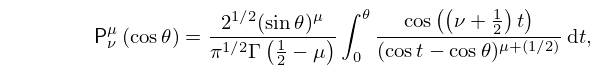
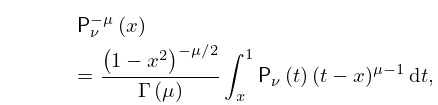
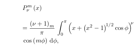
21: 14.12 Integral Representations

… ►

14.12.1 $${𝖯}_{\nu }^{\mu }\left(\cos \theta \right)=\frac{2^{1/2}{(\sin \theta )}^{\mu }}{{\pi }^{1/2}\mathrm{\Gamma }\left(\frac{1}{2}-\mu \right)}{\int }_0^{\theta }\frac{\cos \left(\left(\nu +\frac{1}{2}\right)t\right)}{{(\cos t-\cos \theta )}^{\mu +(1/2)}}dt,$$ , .

ⓘ

Symbols:

$\mathrm{\Gamma }\left(z\right)$: gamma function, : Ferrers function of the first kind, $\pi$: the ratio of the circumference of a circle to its diameter, $\cos z$: cosine function, $dx$: differential of $x$ , $\int$: integral, $\mathrm{\Re }$: real part, $\sin z$: sine function, $\mu$: general order and $\nu$: general degree

Referenced by:

§14.20(iv), §18.10(i)

Permalink:

http://dlmf.nist.gov/14.12.E1

Encodings:

pMML, png, TeX

See also:

Annotations for §14.12(i), §14.12(i), §14.12 and Ch.14

►

14.12.2 $${𝖯}_{\nu }^{-\mu }\left(x\right)=\frac{{\left(1-x^2\right)}^{-\mu /2}}{\mathrm{\Gamma }\left(\mu \right)}{\int }_x^1{𝖯}_{\nu }\left(t\right){(t-x)}^{\mu -1}dt,$$ $\mathrm{\Re }\mu >0$;

ⓘ

Symbols:

$\mathrm{\Gamma }\left(z\right)$: gamma function, : Ferrers function of the first kind, $dx$: differential of $x$ , $\int$: integral, $\mathrm{\Re }$: real part, ${𝖯}_{\nu }\left(x\right)={𝖯}_{\nu }^0\left(x\right)$: Ferrers function of the first kind, $x$: real variable, $\mu$: general order and $\nu$: general degree

Referenced by:

§14.17(i)

Permalink:

http://dlmf.nist.gov/14.12.E2

Encodings:

pMML, png, TeX

See also:

Annotations for §14.12(i), §14.12(i), §14.12 and Ch.14

… ►

14.12.4 $$P_{\nu }^{-\mu }\left(x\right)=\frac{2^{1/2}\mathrm{\Gamma }\left(\mu +\frac{1}{2}\right){\left(x^2-1\right)}^{\mu /2}}{{\pi }^{1/2}\mathrm{\Gamma }\left(\nu +\mu +1\right)\mathrm{\Gamma }\left(\mu -\nu \right)}{\int }_0^{\mathrm{\infty }}\frac{\cosh \left(\left(\nu +\frac{1}{2}\right)t\right)}{{(x+\cosh t)}^{\mu +(1/2)}}dt,$$ $\nu +\mu \ne -1,-2,-3,\mathrm{\dots }$, $\mathrm{\Re }\left(\mu -\nu \right)>0$.

ⓘ

Symbols:

$\mathrm{\Gamma }\left(z\right)$: gamma function, $P_{\nu }^{\mu }\left(z\right)$: associated Legendre function of the first kind, $\pi$: the ratio of the circumference of a circle to its diameter, $dx$: differential of $x$ , $\cosh z$: hyperbolic cosine function, $\int$: integral, $\mathrm{\Re }$: real part, $x$: real variable, $\mu$: general order and $\nu$: general degree

Permalink:

http://dlmf.nist.gov/14.12.E4

Encodings:

pMML, png, TeX

See also:

Annotations for §14.12(ii), §14.12 and Ch.14

►

14.12.5 $$P_{\nu }^{-\mu }\left(x\right)=\frac{{\left(x^2-1\right)}^{-\mu /2}}{\mathrm{\Gamma }\left(\mu \right)}{\int }_1^x{P}_{\nu }\left(t\right){(x-t)}^{\mu -1}dt,$$ $\mathrm{\Re }\mu >0$.

ⓘ

Symbols:

$\mathrm{\Gamma }\left(z\right)$: gamma function, $P_{\nu }^{\mu }\left(z\right)$: associated Legendre function of the first kind, $P_n\left(x\right)$: Legendre polynomial, $dx$: differential of $x$ , $\int$: integral, $\mathrm{\Re }$: real part, $x$: real variable, $\mu$: general order and $\nu$: general degree

Referenced by:

§14.17(i)

Permalink:

http://dlmf.nist.gov/14.12.E5

Encodings:

pMML, png, TeX

See also:

Annotations for §14.12(ii), §14.12 and Ch.14

… ►

14.12.7 $$P_{\nu }^m\left(x\right)=\frac{{\left(\nu +1\right)}_m}{\pi }{\int }_0^{\pi }{\left(x+{\left(x^2-1\right)}^{1/2}\cos \varphi \right)}^{\nu }\cos \left(m\varphi \right)d\varphi ,$$

ⓘ

Symbols:

$P_{\nu }^{\mu }\left(z\right)$: associated Legendre function of the first kind, ${\left(a\right)}_n$: Pochhammer’s symbol (or shifted factorial), $\pi$: the ratio of the circumference of a circle to its diameter, $\cos z$: cosine function, $dx$: differential of $x$ , $\int$: integral, $x$: real variable, $m$: nonnegative integer and $\nu$: general degree

Permalink:

http://dlmf.nist.gov/14.12.E7

Encodings:

pMML, png, TeX

See also:

Annotations for §14.12(ii), §14.12 and Ch.14

…

22: 14.16 Zeros

… ►Throughout this section we assume that $\mu$ and $\nu$ are real, and when they are not integers we write …where $m$, $n\in \mathbb{Z}$ and ${\delta }_{\mu }$, ${\delta }_{\nu }\in (0,1)$. … ►

$\mu >0$, $\mu >\nu$, $\mu \notin \mathbb{Z}$, and $\sin \left((\mu -\nu )\pi \right)$ and $\sin \left(\mu \pi \right)$ have opposite signs.

►

$\mu \le \nu$, $\mu \notin \mathbb{Z}$, and $\lfloor \mu \rfloor$ is odd.

…

23: 14.15 Uniform Asymptotic Approximations

… ►

14.15.1 $${𝖯}_{\nu }^{-\mu }\left(\pm x\right)={\left(\frac{1\mp x}{1\pm x}\right)}^{\mu /2}\left(\sum _{j=0}^{J-1}\frac{{\left(\nu +1\right)}_j{\left(-\nu \right)}_j}{j!\mathrm{\Gamma }\left(j+1+\mu \right)}{\left(\frac{1\mp x}{2}\right)}^j+O\left(\frac{1}{\mathrm{\Gamma }\left(J+1+\mu \right)}\right)\right)$$

ⓘ

Symbols:

$O\left(x\right)$: order not exceeding, $\mathrm{\Gamma }\left(z\right)$: gamma function, : Ferrers function of the first kind, ${\left(a\right)}_n$: Pochhammer’s symbol (or shifted factorial), $!$: factorial (as in $n!$), $x$: real variable, $\mu$: general order, $\nu$: general degree and $J$: nonnegative integer

Referenced by:

§14.15(i)

Permalink:

http://dlmf.nist.gov/14.15.E1

Encodings:

pMML, png, TeX

See also:

Annotations for §14.15(i), §14.15 and Ch.14

…

24: 18.27 $q$-Hahn Class

… ►The $q$-Hahn class OP’s comprise systems of OP’s $\{p_n(x)\}$, $n=0,1,\mathrm{\dots },N$, or $n=0,1,2,\mathrm{\dots }$, that are eigenfunctions of a second order $q$-difference operator. … ►

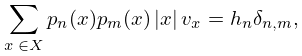
18.27.1 $$A(x)p_n(qx)+B(x)p_n(x)+C(x)p_n(q^{-1}x)={\lambda }_n{p}_n(x),$$

ⓘ

Symbols:

$p_n(x)$: polynomial of degree $n$ , $q$: real variable, $n$: nonnegative integer, $x$: real variable, $A(x)$: coefficient, $C(x)$: coefficient, $C(x)$: coefficient and ${\lambda }_n$: eigenvalue

Referenced by:

§18.28(i)

Permalink:

http://dlmf.nist.gov/18.27.E1

Encodings:

pMML, png, TeX

See also:

Annotations for §18.27(i), §18.27 and Ch.18

… ►

18.27.2 $$\sum _{x\in X}{p}_n(x)p_m(x)|x|v_x=h_n{\delta }_{n,m},$$

ⓘ

Defines:

$v_x$ (locally)

Symbols:

${\delta }_{j,k}$: Kronecker delta, $\in$: element of, $p_n(x)$: polynomial of degree $n$ , $X$: subset of $ℝ$ , $m$: nonnegative integer, $n$: nonnegative integer, $x$: real variable and $h_n$

Referenced by:

§18.27(i), §18.27(i), §18.27(iii)

Permalink:

http://dlmf.nist.gov/18.27.E2

Encodings:

pMML, png, TeX

See also:

Annotations for §18.27(i), §18.27 and Ch.18

… ►Here $a,b$ are fixed positive real numbers, and $I_{+}$ and $I_{-}$ are sequences of successive integers, finite or unbounded in one direction, or unbounded in both directions. … ►

18.27.7 $$p_n(x)=P_n(x;a,b,c;q),$$

ⓘ

Symbols:

$P_n(x;a,b,c;q)$: big $q$-Jacobi polynomial, $p_n(x)$: polynomial of degree $n$ , $q$: real variable, $n$: nonnegative integer and $x$: real variable

Permalink:

http://dlmf.nist.gov/18.27.E7

Encodings:

pMML, png, TeX

See also:

Annotations for §18.27(iii), §18.27 and Ch.18

…

25: 10.41 Asymptotic Expansions for Large Order

§10.41 Asymptotic Expansions for Large Order

►

§10.41(i) Asymptotic Forms

… ►

§10.41(ii) Uniform Expansions for Real Variable

… ► … ►

26: 10.20 Uniform Asymptotic Expansions for Large Order

§10.20 Uniform Asymptotic Expansions for Large Order

… ►In the following formulas for the coefficients $A_k(\zeta )$, $B_k(\zeta )$, $C_k(\zeta )$, and $D_k(\zeta )$, $u_k$, $v_k$ are the constants defined in §9.7(i), and $U_k(p)$, $V_k(p)$ are the polynomials in $p$ of degree $3k$ defined in §10.41(ii). … ► ►

§10.20(iii) Double Asymptotic Properties

►For asymptotic properties of the expansions (10.20.4)–(10.20.6) with respect to large values of $z$ see §10.41(v).

27: 18.3 Definitions

… ►

As eigenfunctions of second order differential operators (Bochner’s theorem, Bochner (1929)). See the differential equations $A(x)p_n^{\prime \prime }(x)+B(x)p_n^{\prime }(x)+{\lambda }_n{p}_n(x)=0$, in Table 18.8.1.

►

With the property that ${\{p_{n+1}^{\prime }(x)\}}_{n=0}^{\mathrm{\infty }}$ is again a system of OP’s. See §18.9(iii).

… ►

18.3.1 $$\sum _{n=1}^{N+1}{T}_j\left(x_{N+1,n}\right)T_k\left(x_{N+1,n}\right)=0,$$ $0\le j\le N$, $0\le k\le N$, $j\ne k$,

ⓘ

Symbols:

$T_n\left(x\right)$: Chebyshev polynomial of the first kind, $N$: positive integer, $n$: nonnegative integer and $x$: real variable

Referenced by:

§18.3, §18.3

Permalink:

http://dlmf.nist.gov/18.3.E1

Encodings:

pMML, png, TeX

See also:

Annotations for §18.3, §18.3 and Ch.18

… ►

18.3.2 $$x_{N+1,n}=\cos \left((n-\frac{1}{2})\pi /(N+1)\right).$$

ⓘ

Symbols:

$\pi$: the ratio of the circumference of a circle to its diameter, $\cos z$: cosine function, $N$: positive integer, $n$: nonnegative integer and $x$: real variable

Permalink:

http://dlmf.nist.gov/18.3.E2

Encodings:

pMML, png, TeX

See also:

Annotations for §18.3, §18.3 and Ch.18

…

28: 24.17 Mathematical Applications

… ►Let ${𝒮}_n$ denote the class of functions that have $n-1$ continuous derivatives on $ℝ$ and are polynomials of degree at most $n$ in each interval $(k,k+1)$, $k\in \mathbb{Z}$. …are called Euler splines of degree $n$. … ► $M_n(x)$ is a monospline of degree $n$, and it follows from (24.4.25) and (24.4.27) that …For each $n=1,2,\mathrm{\dots }$ the function $M_n(x)$ is also the unique cardinal monospline of degree $n$ satisfying (24.17.6), provided that … ►is the unique cardinal monospline of degree $n$ having the least supremum norm ${\Vert F\Vert }_{\mathrm{\infty }}$ on $ℝ$ (minimality property). …

29: 18.28 Askey–Wilson Class

… ► $y$) such that $P_n(z)=p_n(\frac{1}{2}(z+z^{-1}))$ in the Askey–Wilson case, and $P_n(y)=p_n(q^{-y}+c{q}^{y+1})$ in the $q$-Racah case, and both are eigenfunctions of a second order $q$-difference operator similar to (18.27.1). … ►

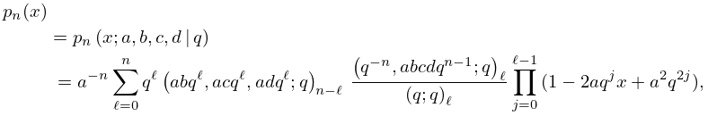
18.28.1 $$p_n(x)=p_n(x;a,b,c,d|q)=a^{-n}\sum _{\mathrm{\ell }=0}^n{q}^{\mathrm{\ell }}{(ab{q}^{\mathrm{\ell }},ac{q}^{\mathrm{\ell }},ad{q}^{\mathrm{\ell }};q)}_{n-\mathrm{\ell }}\frac{{(q^{-n},abcd{q}^{n-1};q)}_{\mathrm{\ell }}}{{(q;q)}_{\mathrm{\ell }}}\prod _{j=0}^{\mathrm{\ell }-1}(1-2a{q}^{j}x+a^2{q}^{2j}),$$

ⓘ

Defines:

$p_n(x;a,b,c,d|q)$: Askey–Wilson polynomial

Symbols:

${(a;q)}_n$: $q$-Pochhammer symbol (or $q$-shifted factorial), ${(a_1,a_2,\mathrm{\dots },a_r;q)}_n$: multiple $q$-Pochhammer symbol, $p_n(x)$: polynomial of degree $n$ , $q$: real variable, $\mathrm{\ell }$: nonnegative integer, $n$: nonnegative integer and $x$: real variable

Referenced by:

(18.28.29), §18.28(ii), §18.38(iii), Erratum (V1.2.0) for Equation (18.28.1)

Permalink:

http://dlmf.nist.gov/18.28.E1

Encodings:

pMML, png, TeX

See also:

Annotations for §18.28(ii), §18.28 and Ch.18

… ►

18.28.2 $${\int }_{-1}^1{p}_n(x)p_m(x)w(x)dx=h_n{\delta }_{n,m},$$ $|a|,|b|,|c|,|d|\le 1$, $ab,ac,ad,bc,bd,cd\ne 1$,

ⓘ

Symbols:

${\delta }_{j,k}$: Kronecker delta, $dx$: differential of $x$ , $\int$: integral, $p_n(x)$: polynomial of degree $n$ , $w(x)$: weight function, $m$: nonnegative integer, $n$: nonnegative integer, $x$: real variable and $h_n$

Referenced by:

Erratum (V1.2.0) for Equation (18.28.2)

Permalink:

http://dlmf.nist.gov/18.28.E2

Encodings:

pMML, png, TeX

Addition (effective with 1.2.0):

This constraint of this equation was updated to include $ab,ac,ad,bc,bd,cd\ne 1$.

See also:

Annotations for §18.28(ii), §18.28(ii), §18.28 and Ch.18

… ►

18.28.6 $${\int }_{-1}^1{p}_n(x)p_m(x)w(x)dx+\sum _{\mathrm{\ell }}{p}_n(x_{\mathrm{\ell }})p_m(x_{\mathrm{\ell }}){\omega }_{\mathrm{\ell }}=h_n{\delta }_{n,m},$$ $ab,ac,ad,bc,bd,cd\in \{z\in ℂ\mid |z|\le 1,z\ne 1\}$,

ⓘ

Symbols:

${\delta }_{j,k}$: Kronecker delta, $ℂ$: complex plane, $dx$: differential of $x$ , $\in$: element of, $\int$: integral, $p_n(x)$: polynomial of degree $n$ , $w(x)$: weight function, $z$: complex variable, $\mathrm{\ell }$: nonnegative integer, $m$: nonnegative integer, $n$: nonnegative integer, $x$: real variable and $h_n$

Referenced by:

Erratum (V1.2.0) for Equation (18.28.6)

Permalink:

http://dlmf.nist.gov/18.28.E6

Encodings:

pMML, png, TeX

Modification (effective with 1.2.0):

This constraint of this equation was updated to include $ab,ac,ad,bc,bd,cd\in \{z\in ℂ\mid |z|\le 1,z\ne 1\}$.

See also:

Annotations for §18.28(ii), §18.28(ii), §18.28 and Ch.18

… ►

18.28.6_5 $$R_n(a^{-1}{q}^{-m};a,b,c,d|q)=R_m({\tilde{a}}^{-1}{q}^{-n};\tilde{a},\tilde{b},\tilde{c},\tilde{d}|q),$$ $m,n=0,1,2,\mathrm{\dots }$.

ⓘ

Symbols:

$q$: real variable, $m$: nonnegative integer and $n$: nonnegative integer

Referenced by:

§18.28(ii), §18.28(ii), Erratum (V1.2.0) Section 18.28

Permalink:

http://dlmf.nist.gov/18.28.E6_5

Encodings:

pMML, png, TeX

Addition (effective with 1.2.0):

This equation was added.

See also:

Annotations for §18.28(ii), §18.28(ii), §18.28 and Ch.18

…

30: 18.36 Miscellaneous Polynomials

… ►Classes of such polynomials have been found that generalize the classical OP’s in the sense that they satisfy second order matrix differential equations with coefficients independent of the degree. … ►This infinite set of polynomials of order $n\ge k$, the smallest power of $x$ being $x^k$ in each polynomial, is a complete orthogonal set with respect to this measure. … ►This lays the foundation for consideration of exceptional OP’s wherein a finite number of (possibly non-sequential) polynomial orders are missing, from what is a complete set even in their absence. … ►Exceptional type I $X_m$-EOP’s, form a complete orthonormal set with respect to a positive measure, but the lowest order polynomial in the set is of order $m$, or, said another way, the first $m$ polynomial orders, $0,1,\mathrm{\dots },m-1$ are missing. The exceptional type III $X_m$-EOP’s are missing orders $1,\mathrm{\dots },m$. …