in two or more variables
(0.006 seconds)
1—10 of 282 matching pages
1: 18.37 Classical OP’s in Two or More Variables
§18.37 Classical OP’s in Two or More Variables
…2: Mark J. Ablowitz
…
►Some of the relationships between IST and Painlevé equations are discussed in two books: Solitons and the Inverse Scattering Transform and Solitons, Nonlinear Evolution Equations and Inverse Scattering.
…
3: Bibliography Y
…
►
Generalized Hypergeometric Functions and Laguerre Polynomials in Two Variables.
In Hypergeometric Functions on Domains of Positivity, Jack
Polynomials, and Applications (Tampa, FL, 1991),
Contemporary Mathematics, Vol. 138, pp. 239–259.
…
4: 1.5 Calculus of Two or More Variables
§1.5 Calculus of Two or More Variables
… ►5: 8.13 Zeros
6: 28.33 Physical Applications
7: Sidebar 21.SB1: Periodic Surface Waves
…
►Two-dimensional periodic waves in a shallow water wave tank.
Taken from Joe Hammack, Daryl McCallister, Norman Scheffner and Harvey Segur, “Two-dimensional periodic waves in shallow water.
…The caption reads “Mosaic of two overhead photographs, showing surface patterns of waves in shallow water”.
…
8: Notices
9: 19.27 Asymptotic Approximations and Expansions
…
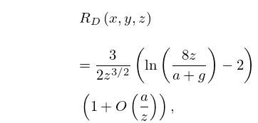
►
19.27.7
.
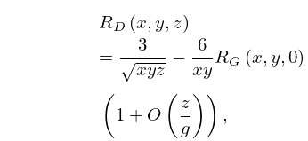
►
19.27.8
.
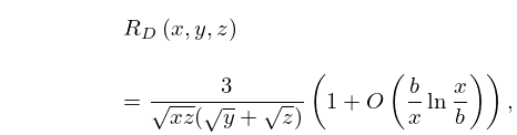
►
19.27.9
.
…
►The approximations in §§19.27(i)–19.27(v) are furnished with upper and lower bounds by Carlson and Gustafson (1994), sometimes with two or three approximations of differing accuracies.
…
►A similar (but more general) situation prevails for when some of the variables
are smaller in magnitude than the rest; see Carlson (1985, (4.16)–(4.19) and (2.26)–(2.29)).
…
