hyperbolic cosecant function

SearchAdvancedHelp

(0.006 seconds)

21—30 of 32 matching pages

21: 19.11 Addition Theorems

… ►

$$\gamma =(({\csc }^2\theta )-{\alpha }^2)(({\csc }^2\varphi )-{\alpha }^2)(({\csc }^2\psi )-{\alpha }^2),$$

… ►

19.11.6_5 $$R_C(\gamma -\delta ,\gamma )=\frac{-1}{\sqrt{\delta }}\arctan \left(\frac{\sqrt{\delta }\sin \theta \sin \varphi \sin \psi }{{\alpha }^2-1-{\alpha }^2\cos \theta \cos \varphi \cos \psi }\right).$$

ⓘ

Symbols:

$R_C(x,y)$: Carlson’s combination of inverse circular and inverse hyperbolic functions, $\cos z$: cosine function, $\arctan z$: arctangent function, $\sin z$: sine function, $\varphi$: real or complex argument, ${\alpha }^2$: real or complex parameter, $\theta$: amplitude, $\psi$: angle, $\gamma$ and $\delta$

Referenced by:

§19.11(i), Erratum (V1.0.28) for Equations (15.2.3_5), (19.11.6_5)

Permalink:

http://dlmf.nist.gov/19.11.E6_5

Encodings:

pMML, png, TeX

Clarification (effective with 1.0.28):

This equation was given a number.

See also:

Annotations for §19.11(i), §19.11 and Ch.19

►Hence, care has to be taken with the multivalued functions in (19.11.5). … ►

$$\gamma =(1-{\alpha }^2)(({\csc }^2\theta )-{\alpha }^2)(({\csc }^2\varphi )-{\alpha }^2),$$

… ►

$$\gamma ={(({\csc }^2\theta )-{\alpha }^2)}^2(({\csc }^2\psi )-{\alpha }^2),$$

…

22: 19.6 Special Cases

… ►

19.6.8 $$F(\varphi ,1)=(\sin \varphi )R_C(1,{\cos }^2\varphi )={\mathrm{gd}}^{-1}\left(\varphi \right).$$

ⓘ

Symbols:

$R_C(x,y)$: Carlson’s combination of inverse circular and inverse hyperbolic functions, $\cos z$: cosine function, $F(\varphi ,k)$: Legendre’s incomplete elliptic integral of the first kind, ${\mathrm{gd}}^{-1}\left(x\right)$: inverse Gudermannian function, $\sin z$: sine function and $\varphi$: real or complex argument

Referenced by:

§19.10(ii), §19.10(ii)

Permalink:

http://dlmf.nist.gov/19.6.E8

Encodings:

pMML, png, TeX

See also:

Annotations for §19.6(ii), §19.6 and Ch.19

►For the inverse Gudermannian function ${\mathrm{gd}}^{-1}\left(\varphi \right)$ see §4.23(viii). … ►Circular and hyperbolic cases, including Cauchy principal values, are unified by using $R_C(x,y)$. Let $c={\csc }^2\varphi \ne {\alpha }^2$ and $\mathrm{\Delta }=\sqrt{1-k^2{\sin }^2\varphi }$. … ►

§19.6(v) $R_C(x,y)$

…

23: 4.15 Graphics

… ►

§4.15(i) Real Arguments

… ►

§4.15(iii) Complex Arguments: Surfaces

►In the graphics shown in this subsection height corresponds to the absolute value of the function and color to the phase. … ►

4.15.3 $$\sec \left(x+\mathrm{i}y\right)=\csc \left(x+\frac{1}{2}\pi +\mathrm{i}y\right),$$

ⓘ

Symbols:

$\pi$: the ratio of the circumference of a circle to its diameter, $\csc z$: cosecant function, $\mathrm{i}$: imaginary unit, $\sec z$: secant function, $x$: real variable and $y$: real variable

Permalink:

http://dlmf.nist.gov/4.15.E3

Encodings:

pMML, png, TeX

See also:

Annotations for §4.15(iii), §4.15 and Ch.4

… ►The corresponding surfaces for $\arccos \left(x+\mathrm{i}y\right)$, $\mathrm{arccot}\left(x+\mathrm{i}y\right)$, $\mathrm{arcsec}\left(x+\mathrm{i}y\right)$ can be visualized from Figures 4.15.9, 4.15.11, 4.15.13 with the aid of equations (4.23.16)–(4.23.18).

24: 1.14 Integral Transforms

… ►The Fourier transform of a real- or complex-valued function $f(t)$ is defined by … ►Suppose $f(t)$ is a real- or complex-valued function and $s$ is a real or complex parameter. … ►

Periodic Functions

… ►The Mellin transform of a real- or complex-valued function $f(x)$ is defined by … ►The Stieltjes transform of a real-valued function $f(t)$ is defined by …

25: 19.8 Quadratic Transformations

… ►

19.8.4 $$\frac{1}{M(a_0,g_0)}=\frac{2}{\pi }{\int }_0^{\pi /2}\frac{d\theta }{\sqrt{a_0^2{\cos }^2\theta +g_0^2{\sin }^2\theta }}=\frac{1}{\pi }{\int }_0^{\mathrm{\infty }}\frac{dt}{\sqrt{t(t+a_0^2)(t+g_0^2)}}.$$

ⓘ

Symbols:

$M(a,g)$: arithmetic-geometric mean, $\pi$: the ratio of the circumference of a circle to its diameter, $\cos z$: cosine function, $dx$: differential of $x$ , $\int$: integral, $\sin z$: sine function, $a_n$: iterate and $g_n$: iterate

Referenced by:

§19.8(i)

Permalink:

http://dlmf.nist.gov/19.8.E4

Encodings:

pMML, png, TeX

See also:

Annotations for §19.8(i), §19.8 and Ch.19

… ►

19.8.14 $$2(k^2-{\alpha }^2)\mathrm{\Pi }(\varphi ,{\alpha }^2,k)=\frac{{\omega }^2-{\alpha }^2}{1+k^{\prime }}\mathrm{\Pi }({\varphi }_1,{\alpha }_1^2,k_1)+k^{2}F(\varphi ,k)-(1+k^{\prime }){\alpha }_1^2{R}_C(c_1,c_1-{\alpha }_1^2),$$

ⓘ

Symbols:

$R_C(x,y)$: Carlson’s combination of inverse circular and inverse hyperbolic functions, $F(\varphi ,k)$: Legendre’s incomplete elliptic integral of the first kind, $\mathrm{\Pi }(\varphi ,{\alpha }^2,k)$: Legendre’s incomplete elliptic integral of the third kind, $\varphi$: real or complex argument, $k$: real or complex modulus, $k^{\prime }$: complementary modulus, ${\alpha }^2$: real or complex parameter, $k_1$: change of variable, ${\varphi }_1$: change of variable, $\omega$: change of variable, ${\alpha }_1$: change of variable and $c_1$: change of variable

Permalink:

http://dlmf.nist.gov/19.8.E14

Encodings:

pMML, png, TeX

See also:

Annotations for §19.8(ii), §19.8(ii), §19.8 and Ch.19

… ►

$c_1={\csc }^2{\varphi }_1.$

… ►

19.8.20 $$\rho \mathrm{\Pi }(\varphi ,{\alpha }^2,k)=\frac{4}{1+k^{\prime }}\mathrm{\Pi }({\psi }_1,{\alpha }_1^2,k_1)+(\rho -1)F(\varphi ,k)-R_C(c-1,c-{\alpha }^2),$$

ⓘ

Symbols:

$R_C(x,y)$: Carlson’s combination of inverse circular and inverse hyperbolic functions, $F(\varphi ,k)$: Legendre’s incomplete elliptic integral of the first kind, $\mathrm{\Pi }(\varphi ,{\alpha }^2,k)$: Legendre’s incomplete elliptic integral of the third kind, $\varphi$: real or complex argument, $k$: real or complex modulus, $k^{\prime }$: complementary modulus, ${\alpha }^2$: real or complex parameter, $k_1$: change of variable, ${\psi }_1$: change of variable, $\rho$: change of variable, ${\alpha }_1^2$: change of variable and $c$: change of variable

Referenced by:

§19.36(ii)

Permalink:

http://dlmf.nist.gov/19.8.E20

Encodings:

pMML, png, TeX

See also:

Annotations for §19.8(iii), §19.8 and Ch.19

… ►

$c={\csc }^2\varphi .$

…

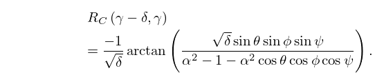
26: 19.16 Definitions

… ►

§19.16(ii) $R_{-a}(𝐛;𝐳)$

… ►The $R$-function is often used to make a unified statement of a property of several elliptic integrals. …where $\mathrm{B}(x,y)$ is the beta function (§5.12) and … ►For generalizations and further information, especially representation of the $R$-function as a Dirichlet average, see Carlson (1977b). …

27: 11.5 Integral Representations

… ►

§11.5(i) Integrals Along the Real Line

… ►

§11.5(ii) Contour Integrals

… ►

Mellin–Barnes Integrals

►

11.5.8 $${(\frac{1}{2}x)}^{-\nu -1}{𝐇}_{\nu }\left(x\right)=-\frac{1}{2\pi \mathrm{i}}{\int }_{-\mathrm{i}\mathrm{\infty }}^{\mathrm{i}\mathrm{\infty }}\frac{\pi \csc \left(\pi s\right)}{\mathrm{\Gamma }\left(\frac{3}{2}+s\right)\mathrm{\Gamma }\left(\frac{3}{2}+\nu +s\right)}{(\frac{1}{4}{x}^2)}^{s}ds,$$ $x>0$, $\mathrm{\Re }\nu >-1$,

ⓘ

Symbols:

$\mathrm{\Gamma }\left(z\right)$: gamma function, ${𝐇}_{\nu }\left(z\right)$: Struve function, $\pi$: the ratio of the circumference of a circle to its diameter, $\csc z$: cosecant function, $dx$: differential of $x$ , $\mathrm{i}$: imaginary unit, $\int$: integral, $\mathrm{\Re }$: real part, $x$: real variable and $\nu$: real or complex order

Keywords:

Mellin transform

Referenced by:

§11.5(ii), §11.5(ii)

Permalink:

http://dlmf.nist.gov/11.5.E8

Encodings:

pMML, png, TeX

See also:

Annotations for §11.5(ii), §11.5(ii), §11.5 and Ch.11

… ►

§11.5(iii) Compendia

…

28: 10.22 Integrals

… ►

§10.22(i) Indefinite Integrals

… ►

Products

… ►

Orthogonality

… ►

Orthogonality

… ►The Hankel transform (or Bessel transform) of a function $f(x)$ is defined as …

29: 22.11 Fourier and Hyperbolic Series

§22.11 Fourier and Hyperbolic Series

… ►

22.11.7 $$\mathrm{ns}(z,k)-\frac{\pi }{2K}\csc \zeta =\frac{2\pi }{K}\sum _{n=0}^{\mathrm{\infty }}\frac{q^{2n+1}\sin \left((2n+1)\zeta \right)}{1-q^{2n+1}},$$

ⓘ

Symbols:

$\mathrm{ns}(z,k)$: Jacobian elliptic function, $\pi$: the ratio of the circumference of a circle to its diameter, $K\left(k\right)$: Legendre’s complete elliptic integral of the first kind, $\csc z$: cosecant function, $q$: nome, $\sin z$: sine function, $z$: complex, $k$: modulus and $\zeta$: change of variable

A&S Ref:

16.23.10

Referenced by:

§22.11

Permalink:

http://dlmf.nist.gov/22.11.E7

Encodings:

pMML, png, TeX

See also:

Annotations for §22.11 and Ch.22

… ►In (22.11.7)–(22.11.12) the left-hand sides are replaced by their limiting values at the poles of the Jacobian functions. … ►A related hyperbolic series is …

30: Errata

… ►

10.22.72 $${\int }_0^{\mathrm{\infty }}{J}_{\mu }\left(at\right)J_{\nu }\left(bt\right)J_{\nu }\left(ct\right)t^{1-\mu }dt=\frac{{(bc)}^{\mu -1}\sin \left((\mu -\nu )\pi \right){(\sinh \chi )}^{\mu -\frac{1}{2}}}{{(\frac{1}{2}{\pi }^3)}^{\frac{1}{2}}{a}^{\mu }}{\mathrm{e}}^{(\mu -\frac{1}{2})\mathrm{i}\pi }{Q}_{\nu -\frac{1}{2}}^{\frac{1}{2}-\mu }\left(\cosh \chi \right),$$ $\mathrm{\Re }\mu >-\frac{1}{2},\mathrm{\Re }\nu >-1,a>b+c,\cosh \chi =(a^2-b^2-c^2)/(2bc)$

Originally, the factor on the right-hand side was written as $\frac{{(bc)}^{\mu -1}\cos \left(\nu \pi \right){(\sinh \chi )}^{\mu -\frac{1}{2}}}{{(\frac{1}{2}{\pi }^3)}^{\frac{1}{2}}{a}^{\mu }}$, which was taken directly from Watson (1944, p. 412, (13.46.5)), who uses a different normalization for the associated Legendre function of the second kind $Q_{\nu }^{\mu }$. Watson’s $Q_{\nu }^{\mu }$ equals $\frac{\sin \left((\nu +\mu )\pi \right)}{\sin \left(\nu \pi \right)}{\mathrm{e}}^{-\mu \pi \mathrm{i}}{Q}_{\nu }^{\mu }$ in the DLMF.

Reported by Arun Ravishankar on 2018-10-22

… ►

Scales were corrected in all figures. The interval $-8.4\le \frac{x-y}{\sqrt{2}}\le 8.4$ was replaced by $-12.0\le \frac{x-y}{\sqrt{2}}\le 12.0$ and $-12.7\le \frac{x+y}{\sqrt{2}}\le 4.2$ replaced by $-18.0\le \frac{x+y}{\sqrt{2}}\le 6.0$. All plots and interactive visualizations were regenerated to improve image quality.

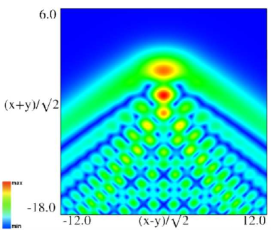
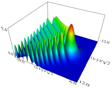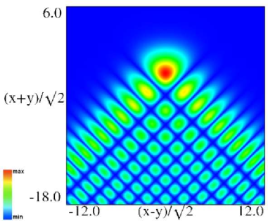
(a) Density plot.	(b) 3D plot.

Figure 36.3.9: Modulus of hyperbolic umbilic canonical integral function $|{\mathrm{\Psi }}^{(\mathrm{H})}\left(x,y,0\right)|$.

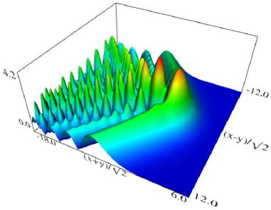
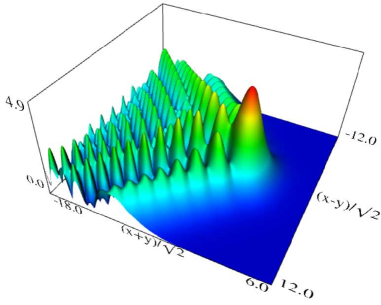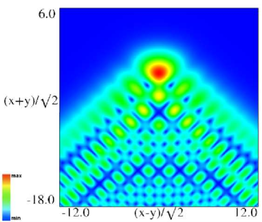
(a) Density plot.	(b) 3D plot.

Figure 36.3.10: Modulus of hyperbolic umbilic canonical integral function $|{\mathrm{\Psi }}^{(\mathrm{H})}\left(x,y,1\right)|$.

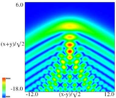
(a) Density plot.	(b) 3D plot.

Figure 36.3.11: Modulus of hyperbolic umbilic canonical integral function $|{\mathrm{\Psi }}^{(\mathrm{H})}\left(x,y,2\right)|$.

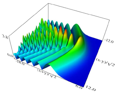(a) Density plot.	(b) 3D plot.

Figure 36.3.12: Modulus of hyperbolic umbilic canonical integral function $|{\mathrm{\Psi }}^{(\mathrm{H})}\left(x,y,3\right)|$.

Reported 2016-09-12 by Dan Piponi.

►

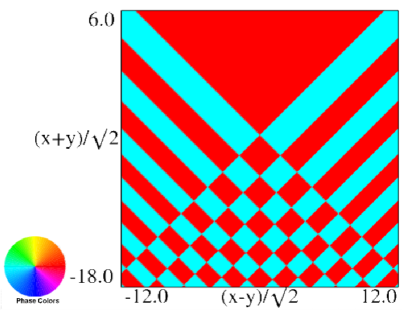
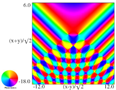
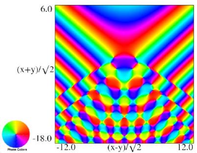
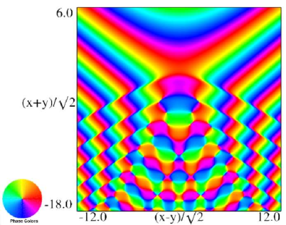
The scaling error reported on 2016-09-12 by Dan Piponi also applied to contour and density plots for the phase of the hyperbolic umbilic canonical integrals. Scales were corrected in all figures. The interval $-8.4\le \frac{x-y}{\sqrt{2}}\le 8.4$ was replaced by $-12.0\le \frac{x-y}{\sqrt{2}}\le 12.0$ and $-12.7\le \frac{x+y}{\sqrt{2}}\le 4.2$ replaced by $-18.0\le \frac{x+y}{\sqrt{2}}\le 6.0$. All plots and interactive visualizations were regenerated to improve image quality.

(a) Contour plot.	(b) Density plot.

Figure 36.3.18: Phase of hyperbolic umbilic canonical integral $\mathrm{ph}{\mathrm{\Psi }}^{(\mathrm{H})}\left(x,y,0\right)$.

(a) Contour plot.	(b) Density plot.

Figure 36.3.19: Phase of hyperbolic umbilic canonical integral $\mathrm{ph}{\mathrm{\Psi }}^{(\mathrm{H})}\left(x,y,1\right)$.

(a) Contour plot.	(b) Density plot.

Figure 36.3.20: Phase of hyperbolic umbilic canonical integral $\mathrm{ph}{\mathrm{\Psi }}^{(\mathrm{H})}\left(x,y,2\right)$.

(a) Contour plot.	(b) Density plot.

Figure 36.3.21: Phase of hyperbolic umbilic canonical integral $\mathrm{ph}{\mathrm{\Psi }}^{(\mathrm{H})}\left(x,y,3\right)$.

Reported 2016-09-28.

… ►

The first paragraph has been rewritten to correct reported errors. The new version is reproduced here.

Let $p$ $(\ne 0)$ and $q$ be real constants and

4.43.1

$A={\left(-\frac{4}{3}p\right)}^{1/2},$

$B={\left(\frac{4}{3}p\right)}^{1/2}.$

The roots of

4.43.2 $$z^3+pz+q=0$$

are:

1. $A\sin a$, $A\sin \left(a+\frac{2}{3}\pi \right)$, and $A\sin \left(a+\frac{4}{3}\pi \right)$, with $\sin \left(3a\right)=4q/A^3$, when $4p^3+27q^2\le 0$.

2. $A\cosh a$, $A\cosh \left(a+\frac{2}{3}\pi \mathrm{i}\right)$, and $A\cosh \left(a+\frac{4}{3}\pi \mathrm{i}\right)$, with $\cosh \left(3a\right)=-4q/A^3$, when , , and $4p^3+27q^2>0$.

3. $B\sinh a$, $B\sinh \left(a+\frac{2}{3}\pi \mathrm{i}\right)$, and $B\sinh \left(a+\frac{4}{3}\pi \mathrm{i}\right)$, with $\sinh \left(3a\right)=-4q/B^3$, when $p>0$.

Note that in Case (a) all the roots are real, whereas in Cases (b) and (c) there is one real root and a conjugate pair of complex roots. See also §1.11(iii).

Reported 2014-10-31 by Masataka Urago.

… ►

Originally the limiting form for $\mathrm{sc}(z,k)$ in the last line of this table was incorrect ($\cosh z$, instead of $\sinh z$).

$\mathrm{sn}(z,k)$ $\to$	$\tanh z$	$\mathrm{cd}(z,k)$ $\to$	$1$	$\mathrm{dc}(z,k)$ $\to$	$1$	$\mathrm{ns}(z,k)$ $\to$	$\coth z$
$\mathrm{cn}(z,k)$ $\to$	$\mathrm{sech}z$	$\mathrm{sd}(z,k)$ $\to$	$\sinh z$	$\mathrm{nc}(z,k)$ $\to$	$\cosh z$	$\mathrm{ds}(z,k)$ $\to$	$\mathrm{csch}z$
$\mathrm{dn}(z,k)$ $\to$	$\mathrm{sech}z$	$\mathrm{nd}(z,k)$ $\to$	$\cosh z$	$\mathrm{sc}(z,k)$ $\to$	$\sinh z$	$\mathrm{cs}(z,k)$ $\to$	$\mathrm{csch}z$

Reported 2010-11-23.

…