hyperbolic%20umbilic%20catastrophe

SearchAdvancedHelp

(0.001 seconds)

11—20 of 230 matching pages

11: 36.7 Zeros

… ►

§36.7(iii) Elliptic Umbilic Canonical Integral

… ►The zeros are lines in $𝐱=(x,y,z)$ space where $\mathrm{ph}{\mathrm{\Psi }}^{(\mathrm{E})}\left(𝐱\right)$ is undetermined. …Near $z=z_n$, and for small $x$ and $y$, the modulus $|{\mathrm{\Psi }}^{(\mathrm{E})}\left(𝐱\right)|$ has the symmetry of a lattice with a rhombohedral unit cell that has a mirror plane and an inverse threefold axis whose $z$ and $x$ repeat distances are given by … ►

§36.7(iv) Swallowtail and Hyperbolic Umbilic Canonical Integrals

►The zeros of these functions are curves in $𝐱=(x,y,z)$ space; see Nye (2007) for ${\mathrm{\Phi }}_3$ and Nye (2006) for ${\mathrm{\Phi }}^{(\mathrm{H})}$.

12: 20 Theta Functions

Chapter 20 Theta Functions

…

13: Bibliography B

… ►

Pionic atoms. Annual Review of Nuclear and Particle Science 20, pp. 467–508.

ⓘ

External Links:

Document

Referenced by:

§33.22(iv).

Encodings:

BibTeX

… ►

A program for computing the Riemann zeta function for complex argument. Comput. Phys. Comm. 20 (3), pp. 441–445.

ⓘ

Notes:

Double-precision Fortran, maximum accuracy 10S.

External Links:

Document, Code, ZentralBlatt

Referenced by:

1st item.

Encodings:

BibTeX

… ►

Coulomb functions (negative energies). Comput. Phys. Comm. 20 (3), pp. 447–458.

ⓘ

Notes:

Double-precision Fortran code.

External Links:

Document, Code

Referenced by:

1st item, 4th item.

Encodings:

BibTeX

… ►

Some solutions of the problem of forced convection. Philos. Mag. Series 7 20, pp. 322–343.

ⓘ

External Links:

Document, ZentralBlatt

Referenced by:

§10.73(iv).

Encodings:

BibTeX

… ►

Bessel functions and modular relations of higher type and hyperbolic differential equations. Comm. Sém. Math. Univ. Lund [Medd. Lunds Univ. Mat. Sem.] 1952 (Tome Supplementaire), pp. 12–20.

ⓘ

External Links:

MathReview (S. C. van Veen), ZentralBlatt

Referenced by:

§35.5(i).

Encodings:

BibTeX

…

14: Bibliography U

… ►

Collisions and umbilic catastrophes. The hyperbolic umbilic canonical diffraction integral. Molecular Phys. 50 (6), pp. 1215–1230.

ⓘ

External Links:

ISSN 0026-8976, Document, MathReview (D. R. J. Chillingworth)

Referenced by:

§36.14(iii).

Encodings:

BibTeX

15: 4.35 Identities

§4.35 Identities

►

§4.35(i) Addition Formulas

… ►

§4.35(ii) Squares and Products

… ►

§4.35(iii) Multiples of the Argument

… ►

§4.35(iv) Real and Imaginary Parts; Moduli

…

16: 4.29 Graphics

… ►

§4.29(i) Real Arguments

… ►

►►

Figure 4.29.6: Principal values of $\mathrm{arccsch}x$ and $\mathrm{arcsech}x$. … Magnify

►

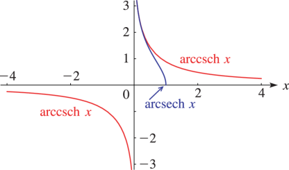§4.29(ii) Complex Arguments

►The conformal mapping $w=\sinh z$ is obtainable from Figure 4.15.7 by rotating both the $w$-plane and the $z$-plane through an angle $\frac{1}{2}\pi$, compare (4.28.8). ►The surfaces for the complex hyperbolic and inverse hyperbolic functions are similar to the surfaces depicted in §4.15(iii) for the trigonometric and inverse trigonometric functions. …

17: 4.28 Definitions and Periodicity

§4.28 Definitions and Periodicity

… ►

Relations to Trigonometric Functions

… ►As a consequence, many properties of the hyperbolic functions follow immediately from the corresponding properties of the trigonometric functions. ►

Periodicity and Zeros

►The functions $\sinh z$ and $\cosh z$ have period $2\pi \mathrm{i}$, and $\tanh z$ has period $\pi \mathrm{i}$. …

18: 4.1 Special Notation

… ► ►►

$k,m,n$	integers.
…

… ►The main purpose of the present chapter is to extend these definitions and properties to complex arguments $z$. … ►; the hyperbolic trigonometric (or just hyperbolic) functions $\sinh z$, $\cosh z$, $\tanh z$, $\mathrm{csch}z$, $\mathrm{sech}z$, $\coth z$; the inverse hyperbolic functions $\mathrm{arcsinh}z$, $\mathrm{Arcsinh}z$, etc. …

19: Errata

… ►

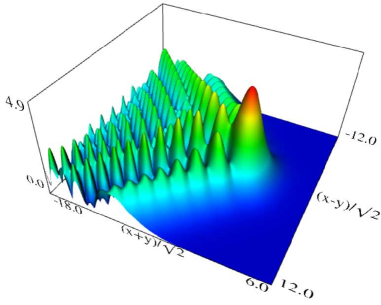
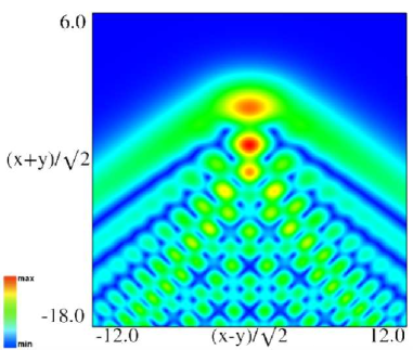
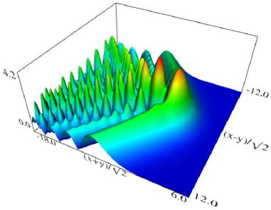
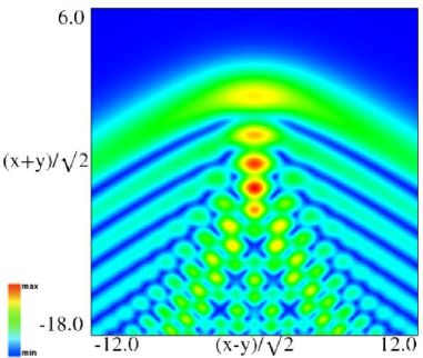
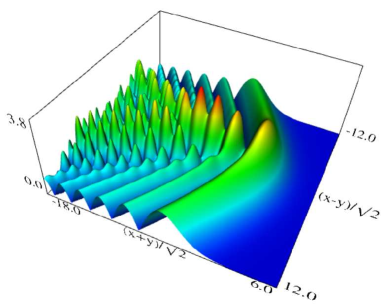
Scales were corrected in all figures. The interval $-8.4\le \frac{x-y}{\sqrt{2}}\le 8.4$ was replaced by $-12.0\le \frac{x-y}{\sqrt{2}}\le 12.0$ and $-12.7\le \frac{x+y}{\sqrt{2}}\le 4.2$ replaced by $-18.0\le \frac{x+y}{\sqrt{2}}\le 6.0$. All plots and interactive visualizations were regenerated to improve image quality.

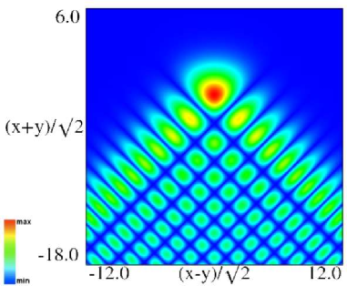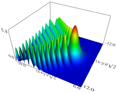(a) Density plot.	(b) 3D plot.

Figure 36.3.9: Modulus of hyperbolic umbilic canonical integral function $|{\mathrm{\Psi }}^{(\mathrm{H})}\left(x,y,0\right)|$.

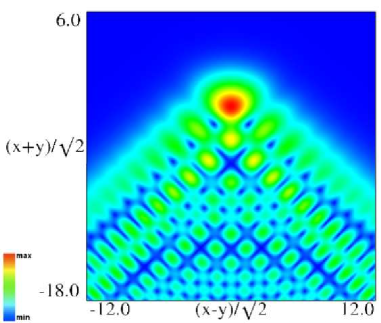(a) Density plot.	(b) 3D plot.

Figure 36.3.10: Modulus of hyperbolic umbilic canonical integral function $|{\mathrm{\Psi }}^{(\mathrm{H})}\left(x,y,1\right)|$.

(a) Density plot.	(b) 3D plot.

Figure 36.3.11: Modulus of hyperbolic umbilic canonical integral function $|{\mathrm{\Psi }}^{(\mathrm{H})}\left(x,y,2\right)|$.

(a) Density plot.	(b) 3D plot.

Figure 36.3.12: Modulus of hyperbolic umbilic canonical integral function $|{\mathrm{\Psi }}^{(\mathrm{H})}\left(x,y,3\right)|$.

Reported 2016-09-12 by Dan Piponi.

►

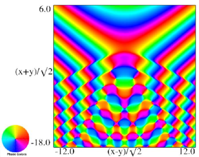
The scaling error reported on 2016-09-12 by Dan Piponi also applied to contour and density plots for the phase of the hyperbolic umbilic canonical integrals. Scales were corrected in all figures. The interval $-8.4\le \frac{x-y}{\sqrt{2}}\le 8.4$ was replaced by $-12.0\le \frac{x-y}{\sqrt{2}}\le 12.0$ and $-12.7\le \frac{x+y}{\sqrt{2}}\le 4.2$ replaced by $-18.0\le \frac{x+y}{\sqrt{2}}\le 6.0$. All plots and interactive visualizations were regenerated to improve image quality.

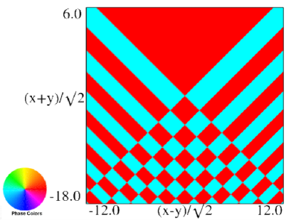(a) Contour plot.	(b) Density plot.

Figure 36.3.18: Phase of hyperbolic umbilic canonical integral $\mathrm{ph}{\mathrm{\Psi }}^{(\mathrm{H})}\left(x,y,0\right)$.

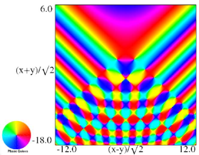(a) Contour plot.	(b) Density plot.

Figure 36.3.19: Phase of hyperbolic umbilic canonical integral $\mathrm{ph}{\mathrm{\Psi }}^{(\mathrm{H})}\left(x,y,1\right)$.

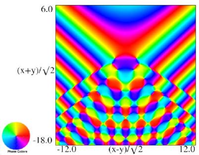(a) Contour plot.	(b) Density plot.

Figure 36.3.20: Phase of hyperbolic umbilic canonical integral $\mathrm{ph}{\mathrm{\Psi }}^{(\mathrm{H})}\left(x,y,2\right)$.

(a) Contour plot.	(b) Density plot.

Figure 36.3.21: Phase of hyperbolic umbilic canonical integral $\mathrm{ph}{\mathrm{\Psi }}^{(\mathrm{H})}\left(x,y,3\right)$.

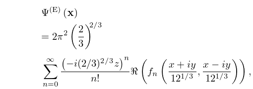
Reported 2016-09-28.

… ►

Several new equations have been added. See (8.17.24), (20.7.34), §20.11(v), (26.12.27), (36.2.28), and (36.2.29).

… ►

36.10.14 $$3\left(\frac{{\partial }^2{\mathrm{\Psi }}^{(\mathrm{E})}}{{\partial x}^2}-\frac{{\partial }^2{\mathrm{\Psi }}^{(\mathrm{E})}}{{\partial y}^2}\right)+2\mathrm{i}z\frac{\partial {\mathrm{\Psi }}^{(\mathrm{E})}}{\partial x}-x{\mathrm{\Psi }}^{(\mathrm{E})}=0$$

Originally this equation appeared with $\frac{\partial {\mathrm{\Psi }}^{(\mathrm{H})}}{\partial x}$ in the second term, rather than $\frac{\partial {\mathrm{\Psi }}^{(\mathrm{E})}}{\partial x}$.

Reported 2010-04-02.

… ►

Bibliographic citations were added in §§1.13(v), 10.14, 10.21(ii), 18.15(v), 18.32, 30.16(iii), 32.13(ii), and as general references in Chapters 19, 20, 22, and 23.

…

20: 36.8 Convergent Series Expansions

§36.8 Convergent Series Expansions

… ►

36.8.3 $$\frac{3^{2/3}}{4{\pi }^2}{\mathrm{\Psi }}^{(\mathrm{H})}\left(3^{1/3}𝐱\right)=\mathrm{Ai}\left(x\right)\mathrm{Ai}\left(y\right)\sum _{n=0}^{\mathrm{\infty }}{(-3^{-1/3}\mathrm{i}z)}^n\frac{c_n(x)c_n(y)}{n!}+\mathrm{Ai}\left(x\right){\mathrm{Ai}}^{\prime }\left(y\right)\sum _{n=2}^{\mathrm{\infty }}{(-3^{-1/3}\mathrm{i}z)}^n\frac{c_n(x)d_n(y)}{n!}+{\mathrm{Ai}}^{\prime }\left(x\right)\mathrm{Ai}\left(y\right)\sum _{n=2}^{\mathrm{\infty }}{(-3^{-1/3}\mathrm{i}z)}^n\frac{d_n(x)c_n(y)}{n!}+{\mathrm{Ai}}^{\prime }\left(x\right){\mathrm{Ai}}^{\prime }\left(y\right)\sum _{n=1}^{\mathrm{\infty }}{(-3^{-1/3}\mathrm{i}z)}^n\frac{d_n(x)d_n(y)}{n!},$$

ⓘ

Symbols:

$\mathrm{Ai}\left(z\right)$: Airy function, $\pi$: the ratio of the circumference of a circle to its diameter, $!$: factorial (as in $n!$), ${\mathrm{\Psi }}^{(\mathrm{H})}\left(𝐱\right)$: hyperbolic umbilic canonical integral function, $\mathrm{i}$: imaginary unit, $y$: real parameter, $z$: real parameter, $m$: integer, $x$: real parameter, $c_n(t)$: coefficients and $d_n(t)$: coefficients

Referenced by:

§36.8

Permalink:

http://dlmf.nist.gov/36.8.E3

Encodings:

pMML, png, TeX

See also:

Annotations for §36.8 and Ch.36

… ►

36.8.4 $${\mathrm{\Psi }}^{(\mathrm{E})}\left(𝐱\right)=2{\pi }^2{\left(\frac{2}{3}\right)}^{2/3}\sum _{n=0}^{\mathrm{\infty }}\frac{{\left(-\mathrm{i}{(2/3)}^{2/3}z\right)}^n}{n!}\mathrm{\Re }\left(f_n(\frac{x+\mathrm{i}y}{{12}^{1/3}},\frac{x-\mathrm{i}y}{{12}^{1/3}})\right),$$

ⓘ

Symbols:

$\pi$: the ratio of the circumference of a circle to its diameter, ${\mathrm{\Psi }}^{(\mathrm{E})}\left(𝐱\right)$: elliptic umbilic canonical integral function, $!$: factorial (as in $n!$), $\mathrm{i}$: imaginary unit, $\mathrm{\Re }$: real part, $y$: real parameter, $z$: real parameter, $m$: integer, $x$: real parameter and $f_n$: function

Referenced by:

§36.8

Permalink:

http://dlmf.nist.gov/36.8.E4

Encodings:

pMML, png, TeX

See also:

Annotations for §36.8 and Ch.36

…