fundamental theorem of arithmetic

SearchAdvancedHelp

(0.000 seconds)

31—40 of 166 matching pages

31: 30.10 Series and Integrals

… ►For an addition theorem, see Meixner and Schäfke (1954, p. 300) and King and Van Buren (1973). …

32: 1.9 Calculus of a Complex Variable

… ►

Arithmetic Operations

… ►

DeMoivre’s Theorem

… ►

Cauchy’s Theorem

… ►

Liouville’s Theorem

… ►

Dominated Convergence Theorem

…

33: 10.44 Sums

… ►

§10.44(i) Multiplication Theorem

… ►

§10.44(ii) Addition Theorems

►

Neumann’s Addition Theorem

… ►

Graf’s and Gegenbauer’s Addition Theorems

…

34: 18.38 Mathematical Applications

… ►Classical OP’s play a fundamental role in Gaussian quadrature. … ►

18.38.3 $$\sum _{m=0}^n{P}_m^{(\alpha ,0)}\left(x\right)=\frac{{\left(\alpha +2\right)}_n}{n!}{}_3{}^{}F_2^{}(\genfrac{}{}{0pt}{}{-n,n+\alpha +2,\frac{1}{2}(\alpha +1)}{\alpha +1,\frac{1}{2}(\alpha +3)};\frac{1}{2}(1-x))\ge 0,$$ $x\ge -1$, $\alpha \ge -2$, $n=0,1,\mathrm{\dots }$,

ⓘ

Symbols:

${}_p{}^{}F_q^{}(a_1,\mathrm{\dots },a_p;b_1,\mathrm{\dots },b_q;z)$ or ${}_p{}^{}F_q^{}(\genfrac{}{}{0pt}{}{a_1,\mathrm{\dots },a_p}{b_1,\mathrm{\dots },b_q};z)$: alternatively ${}_p{}^{}F_q^{}(𝐚;𝐛;z)$ or ${}_p{}^{}F_q^{}(\genfrac{}{}{0pt}{}{𝐚}{𝐛};z)$
generalized hypergeometric function, $P_n^{(\alpha ,\beta )}\left(x\right)$: Jacobi polynomial, ${\left(a\right)}_n$: Pochhammer’s symbol (or shifted factorial), $!$: factorial (as in $n!$), $m$: nonnegative integer, $n$: nonnegative integer and $x$: real variable

Proved:

Askey and Gasper (1976, Theorem 3, p.717)(proved)

Referenced by:

§18.14(iv), §18.18(viii), Erratum (V1.2.0) for Equation (18.38.3)

Permalink:

http://dlmf.nist.gov/18.38.E3

Encodings:

pMML, png, TeX

Modification (effective with 1.2.0):

This equation was updated to include the value of the sum in terms of the ${}_3{}^{}F_2^{}$ function. Also the constraint was previously $\alpha >-1$.

See also:

Annotations for §18.38(ii), §18.38(ii), §18.38 and Ch.18

…

35: Bibliography O

… ►

Error Analysis of Complex Arithmetic. In Computational Aspects of Complex Analysis (Braunlage, 1982), H. Werner, L. Wuytack, E. Ng, and H. J. Bünger (Eds.), NATO Adv. Sci. Inst. Ser. C: Math. Phys. Sci., Vol. 102, pp. 279–292.

ⓘ

External Links:

MathReview (G. Blanch), ZentralBlatt

Referenced by:

§3.1(v).

Encodings:

BibTeX

… ►

Numerical Computing with IEEE Floating Point Arithmetic. Society for Industrial and Applied Mathematics (SIAM), Philadelphia, PA.

ⓘ

Notes:

Including one theorem, one rule of thumb, and one hundred and one exercises

External Links:

ISBN 0-89871-482-6, MathReview (Jesse L. Barlow), ZentralBlatt

Referenced by:

§3.1(i).

Encodings:

BibTeX

36: 15.10 Hypergeometric Differential Equation

… ►

§15.10(i) Fundamental Solutions

… ►When none of the exponent pairs differ by an integer, that is, when none of $c$, $c-a-b$, $a-b$ is an integer, we have the following pairs $f_1(z)$, $f_2(z)$ of fundamental solutions. … ►(a) If $c$ equals $n=1,2,3,\mathrm{\dots }$, and $a=1,2,\mathrm{\dots },n-1$, then fundamental solutions in the neighborhood of $z=0$ are given by (15.10.2) with the interpretation (15.2.5) for $f_2(z)$. … ► … ►The three pairs of fundamental solutions given by (15.10.2), (15.10.4), and (15.10.6) can be transformed into 18 other solutions by means of (15.8.1), leading to a total of 24 solutions known as Kummer’s solutions. …

37: 20.2 Definitions and Periodic Properties

… ►The four points $(0,\pi ,\pi +\tau \pi ,\tau \pi )$ are the vertices of the fundamental parallelogram in the $z$-plane; see Figure 20.2.1. … ►

…

Figure 20.2.1: $z$-plane. Fundamental parallelogram. …

…

38: 19.35 Other Applications

… ►

§19.35(i) Mathematical

►Generalizations of elliptic integrals appear in analysis of modular theorems of Ramanujan (Anderson et al. (2000)); analysis of Selberg integrals (Van Diejen and Spiridonov (2001)); use of Legendre’s relation (19.7.1) to compute $\pi$ to high precision (Borwein and Borwein (1987, p. 26)). …

39: 22.4 Periods, Poles, and Zeros

… ►

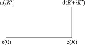
§22.4(ii) Graphical Interpretation via Glaisher’s Notation

►Figure 22.4.2 depicts the fundamental unit cell in the $z$-plane, with vertices $\text{s}=0$, $\text{c}=K$, $\text{d}=K+\mathrm{i}{K}^{\prime }$, $\text{n}=\mathrm{i}{K}^{\prime }$. The set of points $z=mK+n\mathrm{i}{K}^{\prime }$, $m,n\in \mathbb{Z}$, comprise the lattice for the 12 Jacobian functions; all other lattice unit cells are generated by translation of the fundamental unit cell by $mK+n\mathrm{i}{K}^{\prime }$, where again $m,n\in \mathbb{Z}$. ►

►►

Figure 22.4.2: $z$-plane. Fundamental unit cell. Magnify

…

40: 15.17 Mathematical Applications

… ►Quadratic transformations give insight into the relation of elliptic integrals to the arithmetic-geometric mean (§19.22(ii)). … …