functions s(ϵ,ℓ;r),c(ϵ,ℓ;r)

SearchAdvancedHelp

(0.020 seconds)

31—40 of 570 matching pages

31: 11.1 Special Notation

… ►The functions treated in this chapter are the Struve functions ${𝐇}_{\nu }\left(z\right)$ and ${𝐊}_{\nu }\left(z\right)$, the modified Struve functions ${𝐋}_{\nu }\left(z\right)$ and ${𝐌}_{\nu }\left(z\right)$, the Lommel functions $s_{\mu ,\nu }\left(z\right)$ and $S_{\mu ,\nu }\left(z\right)$, the Anger function ${𝐉}_{\nu }\left(z\right)$, the Weber function ${𝐄}_{\nu }\left(z\right)$, and the associated Anger–Weber function ${𝐀}_{\nu }\left(z\right)$.

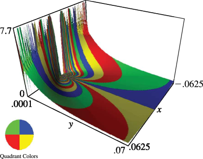
32: 23.16 Graphics

… ►

►

►

Figure 23.16.3: Dedekind’s eta function $\eta \left(x+\mathrm{i}y\right)$ for $-0.0625\le x\le 0.0625$, $0.0001\le y\le 0.07$. Magnify 3D Help

33: 22.1 Special Notation

… ►The functions treated in this chapter are the three principal Jacobian elliptic functions $\mathrm{sn}(z,k)$, $\mathrm{cn}(z,k)$, $\mathrm{dn}(z,k)$; the nine subsidiary Jacobian elliptic functions $\mathrm{cd}(z,k)$, $\mathrm{sd}(z,k)$, $\mathrm{nd}(z,k)$, $\mathrm{dc}(z,k)$, $\mathrm{nc}(z,k)$, $\mathrm{sc}(z,k)$, $\mathrm{ns}(z,k)$, $\mathrm{ds}(z,k)$, $\mathrm{cs}(z,k)$; the amplitude function $\mathrm{am}(x,k)$; Jacobi’s epsilon and zeta functions $ℰ(x,k)$ and $\mathrm{Z}\left(x|k\right)$. … ►Other notations for $\mathrm{sn}(z,k)$ are $\mathrm{sn}(z|m)$ and $\mathrm{sn}(z,m)$ with $m=k^2$; see Abramowitz and Stegun (1964) and Walker (1996). …

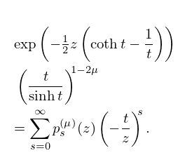
34: 13.24 Series

… ►

13.24.1 $$M_{\kappa ,\mu }\left(z\right)=\mathrm{\Gamma }\left(\kappa +\mu \right)2^{2\kappa +2\mu }{z}^{\frac{1}{2}-\kappa }\sum _{s=0}^{\mathrm{\infty }}{(-1)}^s\frac{{\left(2\kappa +2\mu \right)}_s{\left(2\kappa \right)}_s}{{\left(1+2\mu \right)}_{s}s!}\left(\kappa +\mu +s\right)I_{\kappa +\mu +s}\left(\frac{1}{2}z\right),$$ $2\mu ,\kappa +\mu \ne -1,-2,-3,\mathrm{\dots }$,

ⓘ

Symbols:

$\mathrm{\Gamma }\left(z\right)$: gamma function, ${\left(a\right)}_n$: Pochhammer’s symbol (or shifted factorial), $M_{\kappa ,\mu }\left(z\right)$: Whittaker confluent hypergeometric function, $!$: factorial (as in $n!$), $I_{\nu }\left(z\right)$: modified Bessel function of the first kind, $s$: nonnegative integer and $z$: complex variable

Referenced by:

(13.11.2), §13.24(ii)

Permalink:

http://dlmf.nist.gov/13.24.E1

Encodings:

pMML, png, TeX

See also:

Annotations for §13.24(ii), §13.24 and Ch.13

… ►

13.24.2 $$\frac{1}{\mathrm{\Gamma }\left(1+2\mu \right)}{M}_{\kappa ,\mu }\left(z\right)=2^{2\mu }{z}^{\mu +\frac{1}{2}}\sum _{s=0}^{\mathrm{\infty }}{p}_s^{(\mu )}(z){\left(2\sqrt{\kappa z}\right)}^{-2\mu -s}{J}_{2\mu +s}\left(2\sqrt{\kappa z}\right),$$

ⓘ

Symbols:

$J_{\nu }\left(z\right)$: Bessel function of the first kind, $\mathrm{\Gamma }\left(z\right)$: gamma function, $M_{\kappa ,\mu }\left(z\right)$: Whittaker confluent hypergeometric function, $s$: nonnegative integer, $z$: complex variable and $p_s$: coefficents

Permalink:

http://dlmf.nist.gov/13.24.E2

Encodings:

pMML, png, TeX

See also:

Annotations for §13.24(ii), §13.24 and Ch.13

… ►

13.24.3 $$\exp \left(-\frac{1}{2}z\left(\coth t-\frac{1}{t}\right)\right){\left(\frac{t}{\sinh t}\right)}^{1-2\mu }=\sum _{s=0}^{\mathrm{\infty }}{p}_s^{(\mu )}(z){\left(-\frac{t}{z}\right)}^s.$$

ⓘ

Symbols:

$\exp z$: exponential function, $\coth z$: hyperbolic cotangent function, $\sinh z$: hyperbolic sine function, $s$: nonnegative integer, $z$: complex variable and $p_s$: coefficents

Permalink:

http://dlmf.nist.gov/13.24.E3

Encodings:

pMML, png, TeX

See also:

Annotations for §13.24(ii), §13.24 and Ch.13

…

35: 19.10 Relations to Other Functions

… ►

§19.10(i) Theta and Elliptic Functions

►For relations of Legendre’s integrals to theta functions, Jacobian functions, and Weierstrass functions, see §§20.9(i), 22.15(ii), and 23.6(iv), respectively. … ►

19.10.2 $$(\sinh \varphi )R_C(1,{\cosh }^2\varphi )=\mathrm{gd}\left(\varphi \right).$$

ⓘ

Symbols:

$R_C(x,y)$: Carlson’s combination of inverse circular and inverse hyperbolic functions, $\mathrm{gd}x$: Gudermannian function, $\cosh z$: hyperbolic cosine function, $\sinh z$: hyperbolic sine function and $\varphi$: real or complex argument

Referenced by:

§19.10(ii), §19.6(ii)

Permalink:

http://dlmf.nist.gov/19.10.E2

Encodings:

pMML, png, TeX

See also:

Annotations for §19.10(ii), §19.10 and Ch.19

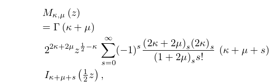
36: 13.1 Special Notation

… ►The main functions treated in this chapter are the Kummer functions $M(a,b,z)$ and $U(a,b,z)$, Olver’s function $𝐌(a,b,z)$, and the Whittaker functions $M_{\kappa ,\mu }\left(z\right)$ and $W_{\kappa ,\mu }\left(z\right)$. …

37: 10.1 Special Notation

… ►For older notations see British Association for the Advancement of Science (1937, pp. xix–xx) and Watson (1944, Chapters 1–3).

38: 25.20 Approximations

… ►

Cody et al. (1971) gives rational approximations for $\zeta \left(s\right)$ in the form of quotients of polynomials or quotients of Chebyshev series. The ranges covered are $0.5\le s\le 5$, $5\le s\le 11$, $11\le s\le 25$, $25\le s\le 55$. Precision is varied, with a maximum of 20S.

►

Piessens and Branders (1972) gives the coefficients of the Chebyshev-series expansions of $s\zeta \left(s+1\right)$ and $\zeta \left(s+k\right)$, $k=2,3,4,5,8$, for $0\le s\le 1$ (23D).

… ►

Antia (1993) gives minimax rational approximations for $\mathrm{\Gamma }\left(s+1\right)F_s(x)$, where $F_s(x)$ is the Fermi–Dirac integral (25.12.14), for the intervals and , with $s=-\frac{1}{2},\frac{1}{2},\frac{3}{2},\frac{5}{2}$. For each $s$ there are three sets of approximations, with relative maximum errors ${10}^{-4},{10}^{-8},{10}^{-12}$.

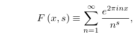
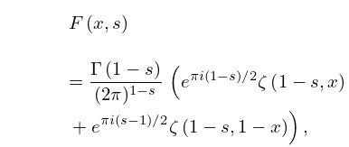
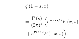
39: 25.13 Periodic Zeta Function

… ►The notation $F(x,s)$ is used for the polylogarithm ${\mathrm{Li}}_s\left({\mathrm{e}}^{2\pi \mathrm{i}x}\right)$ with $x$ real: ►

25.13.1 $$F(x,s)\equiv \sum _{n=1}^{\mathrm{\infty }}\frac{{\mathrm{e}}^{2\pi \mathrm{i}nx}}{n^s},$$

ⓘ

Defines:

$F(x,s)$: periodic zeta function

Symbols:

$\pi$: the ratio of the circumference of a circle to its diameter, $\equiv$: equals by definition, $\mathrm{e}$: base of natural logarithm, $\mathrm{i}$: imaginary unit, $n$: nonnegative integer, $x$: real variable and $s$: complex variable

Keywords:

definition, infinite series, series representation

Source:

Apostol (1976, (9), p. 257)

Permalink:

http://dlmf.nist.gov/25.13.E1

Encodings:

pMML, png, TeX

See also:

Annotations for §25.13 and Ch.25

… ►

25.13.2 $$F(x,s)=\frac{\mathrm{\Gamma }\left(1-s\right)}{{(2\pi )}^{1-s}}\left({\mathrm{e}}^{\pi \mathrm{i}(1-s)/2}\zeta (1-s,x)+{\mathrm{e}}^{\pi \mathrm{i}(s-1)/2}\zeta (1-s,1-x)\right),$$ , $\mathrm{\Re }s>1$,

ⓘ

Symbols:

$\mathrm{\Gamma }\left(z\right)$: gamma function, $\zeta (s,a)$: Hurwitz zeta function, $\pi$: the ratio of the circumference of a circle to its diameter, $\mathrm{e}$: base of natural logarithm, $\mathrm{i}$: imaginary unit, $F(x,s)$: periodic zeta function, $\mathrm{\Re }$: real part, $x$: real variable and $s$: complex variable

Keywords:

connection formula

Source:

Apostol (1976, Exercise 2, p. 273)

Permalink:

http://dlmf.nist.gov/25.13.E2

Encodings:

pMML, png, TeX

See also:

Annotations for §25.13 and Ch.25

►

25.13.3 $$\zeta (1-s,x)=\frac{\mathrm{\Gamma }\left(s\right)}{{(2\pi )}^s}\left({\mathrm{e}}^{-\pi \mathrm{i}s/2}F(x,s)+{\mathrm{e}}^{\pi \mathrm{i}s/2}F(-x,s)\right),$$ $\mathrm{\Re }s>0$ if ; $\mathrm{\Re }s>1$ if $x=1$.

ⓘ

Symbols:

$\mathrm{\Gamma }\left(z\right)$: gamma function, $\zeta (s,a)$: Hurwitz zeta function, $\pi$: the ratio of the circumference of a circle to its diameter, $\mathrm{e}$: base of natural logarithm, $\mathrm{i}$: imaginary unit, $F(x,s)$: periodic zeta function, $\mathrm{\Re }$: real part, $x$: real variable and $s$: complex variable

Keywords:

connection formula

Source:

Apostol (1976, (10), p. 257)

Notes:

This formula is equivalent to (25.11.9).

Referenced by:

Erratum (V1.1.4) for Equation (25.13.3)

Permalink:

http://dlmf.nist.gov/25.13.E3

Encodings:

pMML, png, TeX

See also:

Annotations for §25.13 and Ch.25

40: Simon Ruijsenaars

… ►

28 Mathieu Functions and Hill’s Equation