…
►For large or these series suffer from slow convergence or cancellation (or both).
…
►Quadrature of the integralrepresentations is another effective method.
…
►Lastly, the continued fraction (6.9.1) can be used if is bounded away from the origin.
…
►
…
►Far from the bifurcation set, the leading-order asymptotic formulas of §36.11 reproduce accurately the form of the function, including the geometry of the zeros described in §36.7.
Close to the bifurcation set but far from
, the uniform asymptotic approximations of §36.12 can be used.
…
►(For the umbilics, representations as one-dimensional integrals (§36.2) are used.)
…
►This can be carried out by direct numerical evaluation of canonical integrals along a finite segment of the real axis including all real critical points of , with contributions from the contour outside this range approximated by the first terms of an asymptotic series associated with the endpoints.
…
►For numerical solution of partial differential equations satisfied by the canonical integrals see Connor et al. (1983).
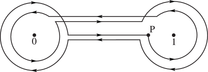
►When
…where the contour starts from an arbitrary point in the interval , circles and then in the positive sense, circles and then in the negative sense, and returns to .
…
►►►Figure 5.12.3:
-plane.
Contour for Pochhammer’s integral.
Magnify
►Many special functions can be represented as a Mellin–Barnes
integral, that is, an integral of a product of gamma functions, reciprocals of gamma functions, and a power of , the integration contour being doubly-infinite and eventually parallel to the imaginary axis at both ends.
…By translating the contour parallel to itself and summing the residues of the integrand, asymptotic expansions of for large , or small , can be obtained complete with an integralrepresentation of the error term.
…
…
►In the case of , for example, this means that in the sectors we may integrate along outward rays from the origin with initial values obtained from §9.2(ii).
But when the integration has to be towards the origin, with starting values of and computed from their asymptotic expansions.
…
►
§9.17(iii) IntegralRepresentations
►Among the integralrepresentations of the Airy functions the Stieltjes transform (9.10.18) furnishes a way of computing in the complex plane, once values of this function can be generated on the positive real axis.
…
►The second method is to apply generalized Gauss–Laguerre quadrature (§3.5(v)) to the integral (9.5.8).
…
 ►
►
