fractional part
(0.001 seconds)
11—20 of 38 matching pages
11: 4.21 Identities
…
►This result is also valid when is fractional or complex, provided that .
…
12: 10.43 Integrals
…
►
§10.43(iii) Fractional Integrals
… ►when and , and by analytic continuation elsewhere. … ►§10.43(iv) Integrals over the Interval ()
… ►When , … ►
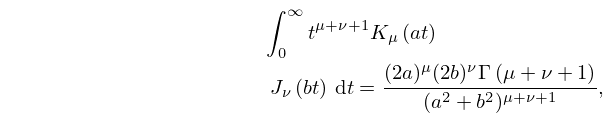
10.43.27
.
…
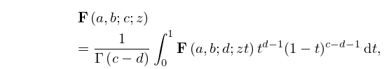
13: 15.6 Integral Representations
…
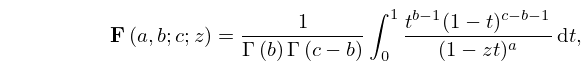
►
15.6.1
; .
►
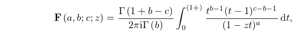
15.6.2
; , .
►
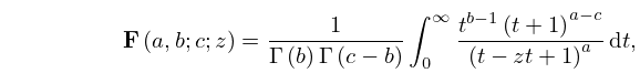
15.6.2_5
; .
…
►
15.6.8
; .
…
►Note that (15.6.8) can be rewritten as a fractional integral.
…
14: 18.40 Methods of Computation
…
►The question is then: how is this possible given only , rather than itself? often converges to smooth results for off the real axis for at a distance greater than the pole spacing of the , this may then be followed by approximate numerical analytic continuation via fitting to lower order continued fractions (either Padé, see §3.11(iv), or pointwise continued fraction approximants, see Schlessinger (1968, Appendix)), to and evaluating these on the real axis in regions of higher pole density that those of the approximating function.
…
15: 15.19 Methods of Computation
…
►For example, in the half-plane we can use (15.12.2) or (15.12.3) to compute and , where is a large positive integer, and then apply (15.5.18) in the backward direction.
When it is better to begin with one of the linear transformations (15.8.4), (15.8.7), or (15.8.8).
…
►
§15.19(v) Continued Fractions
►In Colman et al. (2011) an algorithm is described that uses expansions in continued fractions for high-precision computation of the Gauss hypergeometric function, when the variable and parameters are real and one of the numerator parameters is a positive integer. …16: 33.8 Continued Fractions
§33.8 Continued Fractions
… ►The continued fraction (33.8.1) converges for all finite values of , and (33.8.2) converges for all . ►If we denote and , then …The ambiguous sign in (33.8.4) has to agree with that of the final denominator in (33.8.1) when the continued fraction has converged to the required precision. …17: 4.25 Continued Fractions
§4.25 Continued Fractions
… ►
4.25.2
,
.
…
►See Lorentzen and Waadeland (1992, pp. 560–571) for other continued fractions involving inverse trigonometric functions.
…
18: 18.17 Integrals
…
►
§18.17(iv) Fractional Integrals
►Jacobi
… ►Formulas (18.17.9), (18.17.10) and (18.17.11) are fractional generalizations of -th derivative formulas which are, after substitution of (18.5.7), special cases of (15.5.4), (15.5.5) and (15.5.3), respectively. … ►Formulas (18.17.12) and (18.17.13) are fractional generalizations of the differentiation formulas given in (Erdélyi et al., 1953b, §10.9(15)). ►Laguerre
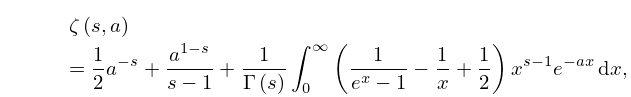
…19: 25.11 Hurwitz Zeta Function
…
►
25.11.27
, , .
…
20: 2.4 Contour Integrals
…
►Except that is now permitted to be complex, with , we assume the same conditions on and also that the Laplace transform in (2.3.8) converges for all sufficiently large values of .
…
►is continuous in and analytic in , and by inversion (§1.14(iii))
…
►in the half-plane .
…Then by integration by parts the integral
…
►However, if , then and different branches of some of the fractional powers of are used for the coefficients ; again see §2.3(iii).
…
