exponential%20growth

SearchAdvancedHelp

(0.002 seconds)

11—20 of 469 matching pages

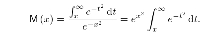
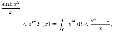
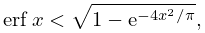
11: 7.8 Inequalities

… ►

7.8.1 $$𝖬\left(x\right)=\frac{{\int }_x^{\mathrm{\infty }}{\mathrm{e}}^{-t^2}dt}{{\mathrm{e}}^{-x^2}}={\mathrm{e}}^{x^2}{\int }_x^{\mathrm{\infty }}{\mathrm{e}}^{-t^2}dt.$$

ⓘ

Defines:

$𝖬\left(x\right)$: Mills’ ratio

Symbols:

$dx$: differential of $x$ , $\mathrm{e}$: base of natural logarithm, $\int$: integral and $x$: real variable

Permalink:

http://dlmf.nist.gov/7.8.E1

Encodings:

pMML, png, TeX

See also:

Annotations for §7.8 and Ch.7

… ►

7.8.6 $a,x>0$.

ⓘ

Symbols:

$dx$: differential of $x$ , $\mathrm{e}$: base of natural logarithm, $\int$: integral and $x$: real variable

Referenced by:

§7.8

Permalink:

http://dlmf.nist.gov/7.8.E6

Encodings:

pMML, png, TeX

See also:

Annotations for §7.8 and Ch.7

►

7.8.7 $x>0$.

ⓘ

Symbols:

$F\left(z\right)$: Dawson’s integral, $dx$: differential of $x$ , $\mathrm{e}$: base of natural logarithm, $\sinh z$: hyperbolic sine function, $\int$: integral and $x$: real variable

Referenced by:

Erratum (V1.1.5) for Additions

Permalink:

http://dlmf.nist.gov/7.8.E7

Encodings:

pMML, png, TeX

Addition (effective with 1.1.5):

A new inequality was added.

See also:

Annotations for §7.8 and Ch.7

►The function $F\left(x\right)/\sqrt{1-{\mathrm{e}}^{-2x^2}}$ is strictly decreasing for $x>0$. … ►

7.8.8 $x>0$.

ⓘ

Symbols:

$\pi$: the ratio of the circumference of a circle to its diameter, $\mathrm{erf}z$: error function, $\mathrm{e}$: base of natural logarithm and $x$: real variable

Source:

Pólya (1949, (1.5))

Referenced by:

§7.8, Erratum (V1.0.17) for Equation (7.8.8)

Permalink:

http://dlmf.nist.gov/7.8.E8

Encodings:

pMML, png, TeX

Addition (effective with 1.0.17):

This inequality was added. It is Pólya (1949, (1.5)). Note that it is a special case of (8.10.11).

Suggested by Roberto Iacono

See also:

Annotations for §7.8 and Ch.7

12: 16.25 Methods of Computation

… ►This occurs when the wanted solution is intermediate in asymptotic growth compared with other solutions. …

13: 7.24 Approximations

… ►

Cody (1969) provides minimax rational approximations for $\mathrm{erf}x$ and $\mathrm{erfc}x$. The maximum relative precision is about 20S.

… ►

Cody et al. (1970) gives minimax rational approximations to Dawson’s integral $F\left(x\right)$ (maximum relative precision 20S–22S).

… ►

Luke (1969b, pp. 323–324) covers $\frac{1}{2}\sqrt{\pi }\mathrm{erf}x$ and ${\mathrm{e}}^{x^2}F\left(x\right)$ for $-3\le x\le 3$ (the Chebyshev coefficients are given to 20D); $\sqrt{\pi }x{\mathrm{e}}^{x^2}\mathrm{erfc}x$ and $2xF\left(x\right)$ for $x\ge 3$ (the Chebyshev coefficients are given to 20D and 15D, respectively). Coefficients for the Fresnel integrals are given on pp. 328–330 (20D).

… ►

Schonfelder (1978) gives coefficients of Chebyshev expansions for $x^{-1}\mathrm{erf}x$ on $0\le x\le 2$, for $x{\mathrm{e}}^{x^2}\mathrm{erfc}x$ on $[2,\mathrm{\infty })$, and for ${\mathrm{e}}^{x^2}\mathrm{erfc}x$ on $[0,\mathrm{\infty })$ (30D).

►

Shepherd and Laframboise (1981) gives coefficients of Chebyshev series for $(1+2x){\mathrm{e}}^{x^2}\mathrm{erfc}x$ on $(0,\mathrm{\infty })$ (22D).

…

14: 20 Theta Functions

Chapter 20 Theta Functions

…

15: 10.75 Tables

… ►

Achenbach (1986) tabulates $J_0\left(x\right)$, $J_1\left(x\right)$, $Y_0\left(x\right)$, $Y_1\left(x\right)$, $x=0(.1)8$, 20D or 18–20S.

… ►

British Association for the Advancement of Science (1937) tabulates $I_0\left(x\right)$, $I_1\left(x\right)$, $x=0(.001)5$, 7–8D; $K_0\left(x\right)$, $K_1\left(x\right)$, $x=0.01(.01)5$, 7–10D; ${\mathrm{e}}^{-x}{I}_0\left(x\right)$, ${\mathrm{e}}^{-x}{I}_1\left(x\right)$, ${\mathrm{e}}^x{K}_0\left(x\right)$, ${\mathrm{e}}^x{K}_1\left(x\right)$, $x=5(.01)10(.1)20$, 8D. Also included are auxiliary functions to facilitate interpolation of the tables of $K_0\left(x\right)$, $K_1\left(x\right)$ for small values of $x$.

►

Bickley et al. (1952) tabulates $x^{-n}{I}_n\left(x\right)$ or ${\mathrm{e}}^{-x}{I}_n\left(x\right)$, $x^n{K}_n\left(x\right)$ or ${\mathrm{e}}^x{K}_n\left(x\right)$, $n=2(1)20$, $x=0$(.01 or .1) 10(.1) 20, 8S; $I_n\left(x\right)$, $K_n\left(x\right)$, $n=0(1)20$, $x=0$ or $0.1(.1)20$, 10S.

… ►

The main tables in Abramowitz and Stegun (1964, Chapter 9) give ${\mathrm{e}}^{-x}{I}_n\left(x\right)$, ${\mathrm{e}}^x{K}_n\left(x\right)$, $n=0,1,2$, $x=0(.1)10(.2)20$, 8D–10D or 10S; $\sqrt{x}{\mathrm{e}}^{-x}{I}_n\left(x\right)$, $(\sqrt{x}/\pi )$ ${\mathrm{e}}^x{K}_n\left(x\right)$, $n=0,1,2$, $1/x=0(.002)0.05$; $K_0\left(x\right)+I_0\left(x\right)\ln x$, $x(K_1\left(x\right)-I_1\left(x\right)\ln x)$, $x=0(.1)2$, 8D; ${\mathrm{e}}^{-x}{I}_n\left(x\right)$, ${\mathrm{e}}^x{K}_n\left(x\right)$, $n=3(1)9$, $x=0(.2)10(.5)20$, 5S; $I_n\left(x\right)$, $K_n\left(x\right)$, $n=0(1)20(10)50,100$, $x=1,2,5,10,50,100$, 9–10S.

… ►

Zhang and Jin (1996, p. 271) tabulates ${\mathrm{e}}^{-x}{\int }_0^x{I}_0\left(t\right)dt$, ${\mathrm{e}}^{-x}{\int }_0^x{t}^{-1}(I_0\left(t\right)-1)dt$, ${\mathrm{e}}^x{\int }_x^{\mathrm{\infty }}{K}_0\left(t\right)dt$, $x{\mathrm{e}}^x{\int }_x^{\mathrm{\infty }}{t}^{-1}{K}_0\left(t\right)dt$, $x=0(.1)1(.5)20$, 8D.

…

16: 25.12 Polylogarithms

… ►When $z={\mathrm{e}}^{\mathrm{i}\theta }$, $0\le \theta \le 2\pi$, (25.12.1) becomes … ►

►►

Figure 25.12.1: Dilogarithm function ${\mathrm{Li}}_2\left(x\right)$, Magnify

►

►

►

Figure 25.12.2: Absolute value of the dilogarithm function $\left|{\mathrm{Li}}_2\left(x+\mathrm{i}y\right)\right|$, $-20\le x\le 20$, $-20\le y\le 20$. … Magnify 3D Help

… ►When $s=2$ and ${\mathrm{e}}^{2\pi \mathrm{i}a}=z$, (25.12.13) becomes (25.12.4). … ►

$F_s(x)=-{\mathrm{Li}}_{s+1}\left(-{\mathrm{e}}^x\right),$

…

17: 7.23 Tables

… ►

Abramowitz and Stegun (1964, Chapter 7) includes $\mathrm{erf}x$, $(2/\sqrt{\pi }){\mathrm{e}}^{-x^2}$, $x\in [0,2]$, 10D; $(2/\sqrt{\pi }){\mathrm{e}}^{-x^2}$, $x\in [2,10]$, 8S; $x{\mathrm{e}}^{x^2}\mathrm{erfc}x$, $x^{-2}\in [0,0.25]$, 7D; $2^n\mathrm{\Gamma }\left(\frac{1}{2}n+1\right){\mathrm{i}}^n\mathrm{erfc}\left(x\right)$, $n=1(1)6,10,11$, $x\in [0,5]$, 6S; $F\left(x\right)$, $x\in [0,2]$, 10D; $xF\left(x\right)$, $x^{-2}\in [0,0.25]$, 9D; $C\left(x\right)$, $S\left(x\right)$, $x\in [0,5]$, 7D; $\mathrm{f}\left(x\right)$, $\mathrm{g}\left(x\right)$, $x\in [0,1]$, $x^{-1}\in [0,1]$, 15D.

… ►

Zhang and Jin (1996, pp. 637, 639) includes $(2/\sqrt{\pi }){\mathrm{e}}^{-x^2}$, $\mathrm{erf}x$, $x=0(.02)1(.04)3$, 8D; $C\left(x\right)$, $S\left(x\right)$, $x=0(.2)10(2)100(100)500$, 8D.

… ►

Zhang and Jin (1996, pp. 638, 640–641) includes the real and imaginary parts of $\mathrm{erf}z$, $x\in [0,5]$, $y=0.5(.5)3$, 7D and 8D, respectively; the real and imaginary parts of ${\int }_x^{\mathrm{\infty }}{\mathrm{e}}^{\pm \mathrm{i}{t}^2}dt$, $(1/\sqrt{\pi }){\mathrm{e}}^{\mp \mathrm{i}(x^2+(\pi /4))}{\int }_x^{\mathrm{\infty }}{\mathrm{e}}^{\pm \mathrm{i}{t}^2}dt$, $x=0(.5)20(1)25$, 8D, together with the corresponding modulus and phase to 8D and 6D (degrees), respectively.

…

18: 2.11 Remainder Terms; Stokes Phenomenon

… ►From §8.19(i) the generalized exponential integral is given by …However, on combining (2.11.6) with the connection formula (8.19.18), with $m=1$, we derive … ►Owing to the factor ${\mathrm{e}}^{-\rho }$, that is, ${\mathrm{e}}^{-|z|}$ in (2.11.13), $F_{n+p}\left(z\right)$ is uniformly exponentially small compared with $E_p\left(z\right)$. … ►A simple example is provided by Euler’s transformation (§3.9(ii)) applied to the asymptotic expansion for the exponential integral (§6.12(i)): … ►For example, using double precision $d_{20}$ is found to agree with (2.11.31) to 13D. …

19: 4.11 Sums

§4.11 Sums

►For infinite series involving logarithms and/or exponentials, see Gradshteyn and Ryzhik (2000, Chapter 1), Hansen (1975, §44), and Prudnikov et al. (1986a, Chapter 5).

20: 9.18 Tables

… ►

Fox (1960, Table 3) tabulates $2{\pi }^{1/2}{x}^{1/4}\exp (\frac{2}{3}{x}^{3/2})\mathrm{Ai}\left(x\right)$, $2{\pi }^{1/2}{x}^{-1/4}\exp (\frac{2}{3}{x}^{3/2}){\mathrm{Ai}}^{\prime }\left(x\right)$, ${\pi }^{1/2}{x}^{1/4}\exp (-\frac{2}{3}{x}^{3/2})\mathrm{Bi}\left(x\right)$, and ${\pi }^{1/2}{x}^{-1/4}\exp (-\frac{2}{3}{x}^{3/2}){\mathrm{Bi}}^{\prime }\left(x\right)$ for $\frac{3}{2}{x}^{-3/2}=0(.001)0.05$, together with similar auxiliary functions for negative values of $x$. Precision is 10D.

►

Zhang and Jin (1996, p. 337) tabulates $\mathrm{Ai}\left(x\right)$, ${\mathrm{Ai}}^{\prime }\left(x\right)$, $\mathrm{Bi}\left(x\right)$, ${\mathrm{Bi}}^{\prime }\left(x\right)$ for $x=0(1)20$ to 8S and for $x=-20(1)0$ to 9D.

… ►

Miller (1946) tabulates $a_k$, ${\mathrm{Ai}}^{\prime }\left(a_k\right)$, $a_k^{\prime }$, $\mathrm{Ai}\left(a_k^{\prime }\right)$, $k=1(1)50$; $b_k$, ${\mathrm{Bi}}^{\prime }\left(b_k\right)$, $b_k^{\prime }$, $\mathrm{Bi}\left(b_k^{\prime }\right)$, $k=1(1)20$. Precision is 8D. Entries for $k=1(1)20$ are reproduced in Abramowitz and Stegun (1964, Chapter 10).

►

Sherry (1959) tabulates $a_k$, ${\mathrm{Ai}}^{\prime }\left(a_k\right)$, $a_k^{\prime }$, $\mathrm{Ai}\left(a_k^{\prime }\right)$, $k=1(1)50$; 20S.

►

Zhang and Jin (1996, p. 339) tabulates $a_k$, ${\mathrm{Ai}}^{\prime }\left(a_k\right)$, $a_k^{\prime }$, $\mathrm{Ai}\left(a_k^{\prime }\right)$, $b_k$, ${\mathrm{Bi}}^{\prime }\left(b_k\right)$, $b_k^{\prime }$, $\mathrm{Bi}\left(b_k^{\prime }\right)$, $k=1(1)20$; 8D.

…