derivative rule

(0.002 seconds)

11—18 of 18 matching pages

12: 3.8 Nonlinear Equations

… ►

§3.8(ii) Newton’s Rule

… ► … ►Newton’s rule is given by … ►Another iterative method is Halley’s rule: …The rule converges locally and is cubically convergent. …

M. J. Gander and A. H. Karp (2001) Stable computation of high order Gauss quadrature rules using discretization for measures in radiation transfer. J. Quant. Spectrosc. Radiat. Transfer 68 (2), pp. 213–223.

ⓘ

Referenced by:: §18.39(iii).
Encodings:: BibTeX

… ►

W. Gautschi (1994) Algorithm 726: ORTHPOL — a package of routines for generating orthogonal polynomials and Gauss-type quadrature rules. ACM Trans. Math. Software 20 (1), pp. 21–62.

ⓘ

Notes:: For remark see same journal 24(1998), p. 355.
External Links:: Document, ISSN 0098-3500, GAMS (module 726; package TOMS), ZentralBlatt
Referenced by:: 2nd item, §3.5(v), §3.5(v).
Encodings:: BibTeX

… ►

A. Gil, J. Segura, and N. M. Temme (2003b) Computing special functions by using quadrature rules. Numer. Algorithms 33 (1-4), pp. 265–275.

ⓘ

Notes:: International Conference on Numerical Algorithms, Vol. I (Marrakesh, 2001)
External Links:: ISSN 1017-1398, Document, MathReview, ZentralBlatt
Referenced by:: §3.5(ix).
Encodings:: BibTeX

… ►

A. Gil and J. Segura (2014) On the complex zeros of Airy and Bessel functions and those of their derivatives. Anal. Appl. (Singap.) 12 (5), pp. 537–561.

ⓘ

External Links:: ISSN 0219-5305, Document, Link, MathReview Entry, ZentralBlatt
Referenced by:: §9.9(i), §9.9(i).
Encodings:: BibTeX

… ►

G. H. Golub and J. H. Welsch (1969) Calculation of Gauss quadrature rules. Math. Comp. 23 (106), pp. 221–230.

ⓘ

Notes:: Loose microfiche suppl. A1–A10
External Links:: FullText, MathReview (F. Stenger), ZentralBlatt
Referenced by:: §18.39(iii), §3.5(vi).
Encodings:: BibTeX

…

14: Bibliography W

… ►

J. Waldvogel (2006) Fast construction of the Fejér and Clenshaw-Curtis quadrature rules. BIT 46 (1), pp. 195–202.

ⓘ

External Links:: ISSN 0006-3835, Document, MathReview Entry, ZentralBlatt
Referenced by:: §3.5(iv).
Encodings:: BibTeX

… ►

P. L. Walker (2007) The zeros of Euler’s psi function and its derivatives. J. Math. Anal. Appl. 332 (1), pp. 607–616.

ⓘ

External Links:: ISSN 0022-247X, Document, MathReview, ZentralBlatt (Mehdi Hassani)
Referenced by:: §5.4(iii).
Encodings:: BibTeX

… ►

R. J. Wells (1999) Rapid approximation to the Voigt/Faddeeva function and its derivatives. J. Quant. Spect. and Rad. Transfer 62 (1), pp. 29–48.

ⓘ

Notes:: Includes Fortran code in the appendices to compute the functions to an accuracy between $10^{-2}$ and $10^{-5}$ .
External Links:: ISSN 0022-4073, Document
Referenced by:: §7.21, §7.21.
Encodings:: BibTeX

…

15: Bibliography

… ►

G. Allasia and R. Besenghi (1987a) Numerical computation of Tricomi’s psi function by the trapezoidal rule. Computing 39 (3), pp. 271–279.

ⓘ

External Links:: ISSN 0010-485X, Document, MathReview, ZentralBlatt
Referenced by:: §13.29(iii).
Encodings:: BibTeX

►

G. Allasia and R. Besenghi (1991) Numerical evaluation of the Kummer function with complex argument by the trapezoidal rule. Rend. Sem. Mat. Univ. Politec. Torino 49 (3), pp. 315–327.

ⓘ

External Links:: ISSN 0373-1243, MathReview, ZentralBlatt
Referenced by:: §13.29(iii).
Encodings:: BibTeX

►

G. Allasia and R. Besenghi (1987b) Numerical calculation of incomplete gamma functions by the trapezoidal rule. Numer. Math. 50 (4), pp. 419–428.

ⓘ

External Links:: ISSN 0029-599X, Document, MathReview (F. W. J. Olver), ZentralBlatt
Referenced by:: §8.25(ii).
Encodings:: BibTeX

►

G. Allasia and R. Besenghi (1989) Numerical Calculation of the Riemann Zeta Function and Generalizations by Means of the Trapezoidal Rule. In Numerical and Applied Mathematics, Part II (Paris, 1988), C. Brezinski (Ed.), IMACS Ann. Comput. Appl. Math., Vol. 1, pp. 467–472.

ⓘ

External Links:: MathReview
Referenced by:: §25.18(i).
Encodings:: BibTeX

… ►

D. E. Amos (1983b) Algorithm 610. A portable FORTRAN subroutine for derivatives of the psi function. ACM Trans. Math. Software 9 (4), pp. 494–502.

ⓘ

Notes:: Single and double precision, maximum accuracy 18S.
External Links:: ISSN 0098-3500, Document, GAMS (module 610; package TOMS), MathReview Entry, ZentralBlatt
Referenced by:: 1st item.
Encodings:: BibTeX

…

16: 3.11 Approximation Techniques

… ►The Padé approximants can be computed by Wynn’s cross rule. Any five approximants arranged in the Padé table as … ►From the equations

\ifrac{\partial S}{\partial a_{k}}=0

k=0,1,\dots,n

, we derive the normal equations … ►Given

n+1

distinct points

x_{k}

in the real interval

[a,b]

, with (

a=

)

x_{0}<x_{1}<\cdots<x_{n-1}<x_{n}

(

=b

), on each subinterval

[x_{k},x_{k+1}]

k=0,1,\ldots,n-1

, a low-degree polynomial is defined with coefficients determined by, for example, values

f_{k}

and

f_{k}^{\prime}

of a function

f

and its derivative at the nodes

x_{k}

and

x_{k+1}

. …By taking more derivatives into account, the smoothness of the spline will increase. …

17: Bibliography T

… ►

N. M. Temme (1979a) An algorithm with ALGOL 60 program for the computation of the zeros of ordinary Bessel functions and those of their derivatives. J. Comput. Phys. 32 (2), pp. 270–279.

ⓘ

External Links:: Document, ZentralBlatt
Referenced by:: §10.74(vi), §10.77(x).
Encodings:: BibTeX

… ►

N. M. Temme (1978) The numerical computation of special functions by use of quadrature rules for saddle point integrals. II. Gamma functions, modified Bessel functions and parabolic cylinder functions. Report TW 183/78 Mathematisch Centrum, Amsterdam, Afdeling Toegepaste Wiskunde.

ⓘ

Notes:: Algol procedures, maximum accuracy 14S.
External Links:: FullText, ZentralBlatt
Referenced by:: §12.21(ii).
Encodings:: BibTeX

…

18: 1.6 Vectors and Vector-Valued Functions

… ►where

\mathbf{n}

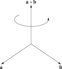
is the unit vector normal to

\mathbf{a}

and

\mathbf{b}

whose direction is determined by the right-hand rule; see Figure 1.6.1. ►

See accompanying text — Figure 1.6.1: Vector notation. Right-hand rule for cross products. Magnify

… ►

1.6.19

\nabla=\mathbf{i}\frac{\partial}{\partial x}+\mathbf{j}\frac{\partial}{% \partial y}+\mathbf{k}\frac{\partial}{\partial z}.

ⓘ

Symbols:: $\frac{\partial\NVar{f}}{\partial\NVar{x}}$ : partial derivative of $f$ with respect to $x$ , $\,\partial\NVar{x}$ : partial differential of $x$ , $z$ : variable, $\mathbf{i}$ : unit vector, $\mathbf{j}$ : unit vector and $\mathbf{k}$ : unit vector
Permalink:: http://dlmf.nist.gov/1.6.E19
Encodings:: pMML, png, TeX
See also:: Annotations for §1.6(iii), §1.6(iii), §1.6 and Ch.1

… ►where

\ifrac{\partial g}{\partial n}=\nabla g\cdot\mathbf{n}

is the derivative of

g

normal to the surface outwards from

V

and

\mathbf{n}

is the unit outer normal vector. …