cosine transform

SearchAdvancedHelp

(0.003 seconds)

1—10 of 56 matching pages

1: 1.14 Integral Transforms

… ►

§1.14(ii) Fourier Cosine and Sine Transforms

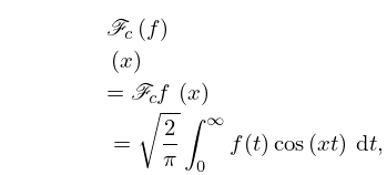
►The Fourier cosine transform and Fourier sine transform are defined respectively by ►

1.14.9 $${ℱ}_c\left(f\right)\left(x\right)={ℱ}_{c}f\left(x\right)=\sqrt{\frac{2}{\pi }}{\int }_0^{\mathrm{\infty }}f(t)\cos \left(xt\right)dt,$$

ⓘ

Defines:

${ℱ}_c\left(f\right)\left(s\right)$: Fourier cosine transform

Symbols:

$\pi$: the ratio of the circumference of a circle to its diameter, $\cos z$: cosine function, $dx$: differential of $x$ , $\int$: integral and $F_c(x)$: cosine transformation of $f(t)$

Referenced by:

§1.17(ii), §1.18(vi), §1.18(vi)

Permalink:

http://dlmf.nist.gov/1.14.E9

Encodings:

pMML, png, TeX

Notational Change (effective with 1.0.15):

This equation defines the general notation ${ℱ}_c\left(f\right)\left(x\right)$ or ${ℱ}_{c}f\left(x\right)$. Previously it defined the local notation $F_c(x)$ used in this subsection.

See also:

Annotations for §1.14(ii), §1.14 and Ch.1

… ►In this subsection we let $F_c(x)={ℱ}_{c}f\left(x\right)$, $F_s(x)={ℱ}_{s}f\left(x\right)$, $G_c(x)={ℱ}_{c}g\left(x\right)$, and $G_s(x)={ℱ}_{s}g\left(x\right)$. … ►

Table 1.14.2: Fourier cosine transforms.

► ►►

$f(t)$	$\sqrt{{\displaystyle \frac{2}{\pi }}}{\displaystyle {\int }_0^{\mathrm{\infty }}}f(t)\cos \left(xt\right)dt$,	$x>0$
…

►

…

2: 15.17 Mathematical Applications

… ►Harmonic analysis can be developed for the Jacobi transform either as a generalization of the Fourier-cosine transform (§1.14(ii)) or as a specialization of a group Fourier transform. …

3: 1.18 Linear Second Order Differential Operators and Eigenfunction Expansions

… ►

Example 2: Sine and Cosine Transforms, $X=[0,\mathrm{\infty })$

►The Fourier cosine and sine transform pairs (1.14.9) & (1.14.11) and (1.14.10) & (1.14.12) can be easily obtained from (1.18.57) as for $\nu =\pm \frac{1}{2}$ the Bessel functions reduce to the trigonometric functions, see (10.16.1). … ►For $f(x)$ even in $x$ this yields the Fourier cosine transform pair (1.14.9) & (1.14.11), and for $f(x)$ odd the Fourier sine transform pair (1.14.10) & (1.14.12). … …

4: Errata

… ►

There have been extensive changes in the notation used for the integral transforms defined in §1.14. These changes are applied throughout the DLMF. The following table summarizes the changes.

Transform	New	Abbreviated	Old
	Notation	Notation	Notation
Fourier	$ℱ\left(f\right)\left(x\right)$	$ℱf\left(x\right)$
Fourier Cosine	${ℱ}_c\left(f\right)\left(x\right)$	${ℱ}_{c}f\left(x\right)$
Fourier Sine	${ℱ}_s\left(f\right)\left(x\right)$	${ℱ}_{s}f\left(x\right)$
Laplace	$ℒ\left(f\right)\left(s\right)$	$ℒf\left(s\right)$	$ℒ(f(t);s)$
Mellin	$ℳ\left(f\right)\left(s\right)$	$ℳf\left(s\right)$	$ℳ(f;s)$
Hilbert	$\mathscr{H}\left(f\right)\left(s\right)$	$\mathscr{H}f\left(s\right)$	$\mathscr{H}(f;s)$
Stieltjes	$𝒮\left(f\right)\left(s\right)$	$𝒮f\left(s\right)$	$𝒮(f;s)$

Previously, for the Fourier, Fourier cosine and Fourier sine transforms, either temporary local notations were used or the Fourier integrals were written out explicitly.

…

5: 6.14 Integrals

… ►

§6.14(i) Laplace Transforms

…

6: 18.3 Definitions

… ►It is also related to a discrete Fourier-cosine transform, see Britanak et al. (2007). …

7: 18.17 Integrals

… ►

18.17.32 $${\int }_0^{\mathrm{\infty }}{\mathrm{e}}^{-ax}{x}^{\nu -1-2n}{L}_{2n}^{(\nu -1-2n)}\left(ax\right)\cos \left(xy\right)dx=\frac{{(-1)}^n\mathrm{\Gamma }\left(\nu \right)}{2(2n)!}{y}^{2n}\left({(a+iy)}^{-\nu }+{(a-iy)}^{-\nu }\right),$$ $\nu >2n$, $a>0$.

ⓘ

Symbols:

$\mathrm{\Gamma }\left(z\right)$: gamma function, $L_n^{(\alpha )}\left(x\right)$: Laguerre (or generalized Laguerre) polynomial, $\cos z$: cosine function, $dx$: differential of $x$ , $\mathrm{e}$: base of natural logarithm, $!$: factorial (as in $n!$), $\int$: integral, $y$: real variable, $n$: nonnegative integer and $x$: real variable

Referenced by:

§18.17(v)

Permalink:

http://dlmf.nist.gov/18.17.E32

Encodings:

pMML, png, TeX

See also:

Annotations for §18.17(v), §18.17(v), §18.17 and Ch.18

…

8: Bibliography B

… ►

Discrete Cosine and Sine Transforms. General Properties, Fast Algorithms and Integer Approximations. Elsevier/Academic Press, Amsterdam.

ⓘ

External Links:

ISBN 978-0-12-373624-6; 0-12-373624-2, MathReview (Gerd Teschke)

Referenced by:

§18.3.

Encodings:

BibTeX

…

9: 19.7 Connection Formulas

… ►

Reciprocal-Modulus Transformation

… ►

Imaginary-Modulus Transformation

… ►

$$E(\varphi ,\mathrm{i}k)=(1/{\kappa }^{\prime })\left(E(\theta ,\kappa )-{\kappa }^2(\sin \theta \cos \theta ){(1-{\kappa }^2{\sin }^2\theta )}^{-1/2}\right),$$

… ►

Imaginary-Argument Transformation

… ►For two further transformations of this type see Erdélyi et al. (1953b, p. 316). …

10: 7.14 Integrals

… ►

7.14.5 $${\int }_0^{\mathrm{\infty }}{\mathrm{e}}^{-at}C\left(t\right)dt=\frac{1}{a}\mathrm{f}\left(\frac{a}{\pi }\right),$$ $\mathrm{\Re }a>0$,

ⓘ

Symbols:

$\mathrm{f}\left(z\right)$: auxiliary function for Fresnel integrals, $C\left(z\right)$: Fresnel integral, $\pi$: the ratio of the circumference of a circle to its diameter, $dx$: differential of $x$ , $\mathrm{e}$: base of natural logarithm, $\int$: integral and $\mathrm{\Re }$: real part

Keywords:

Laplace transform

A&S Ref:

7.4.27 (in different notation)

Referenced by:

§7.14(ii)

Permalink:

http://dlmf.nist.gov/7.14.E5

Encodings:

pMML, png, TeX

See also:

Annotations for §7.14(ii), §7.14(ii), §7.14 and Ch.7

… ►

7.14.7 $${\int }_0^{\mathrm{\infty }}{\mathrm{e}}^{-at}C\left(\sqrt{\frac{2t}{\pi }}\right)dt=\frac{{(\sqrt{a^2+1}+a)}^{\frac{1}{2}}}{2a\sqrt{a^2+1}},$$ $\mathrm{\Re }a>0$,

ⓘ

Symbols:

$C\left(z\right)$: Fresnel integral, $\pi$: the ratio of the circumference of a circle to its diameter, $dx$: differential of $x$ , $\mathrm{e}$: base of natural logarithm, $\int$: integral and $\mathrm{\Re }$: real part

Keywords:

Laplace transform

A&S Ref:

7.4.29 in modified form

Referenced by:

§7.14(ii)

Permalink:

http://dlmf.nist.gov/7.14.E7

Encodings:

pMML, png, TeX

See also:

Annotations for §7.14(ii), §7.14(ii), §7.14 and Ch.7

…