contour integral

SearchAdvancedHelp

(0.003 seconds)

31—40 of 53 matching pages

31: 12.14 The Function $W(a,x)$

… ►These follow from the contour integrals of §12.5(ii), which are valid for general complex values of the argument $z$ and parameter $a$. …

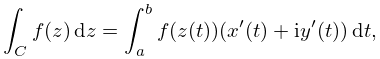
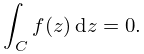
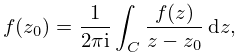
32: 1.9 Calculus of a Complex Variable

… ►

1.9.28 $${\int }_{C}f(z)dz={\int }_a^{b}f(z(t))(x^{\prime }(t)+\mathrm{i}{y}^{\prime }(t))dt,$$

ⓘ

Symbols:

$dx$: differential of $x$ , $\mathrm{i}$: imaginary unit, $\int$: integral and $C$: closed contour

Permalink:

http://dlmf.nist.gov/1.9.E28

Encodings:

pMML, png, TeX

See also:

Annotations for §1.9(iii), §1.9 and Ch.1

… ►

1.9.29 $${\int }_{C}f(z)dz=0.$$

ⓘ

Symbols:

$dx$: differential of $x$ , $\int$: integral and $C$: closed contour

Permalink:

http://dlmf.nist.gov/1.9.E29

Encodings:

pMML, png, TeX

See also:

Annotations for §1.9(iii), §1.9(iii), §1.9 and Ch.1

… ►

1.9.30 $$f(z_0)=\frac{1}{2\pi \mathrm{i}}{\int }_C\frac{f(z)}{z-z_0}dz,$$

ⓘ

Symbols:

$\pi$: the ratio of the circumference of a circle to its diameter, $dx$: differential of $x$ , $\mathrm{i}$: imaginary unit, $\int$: integral and $C$: closed contour

Referenced by:

§2.3(iii)

Permalink:

http://dlmf.nist.gov/1.9.E30

Encodings:

pMML, png, TeX

See also:

Annotations for §1.9(iii), §1.9(iii), §1.9 and Ch.1

… ►

1.9.31 $$f^{(n)}(z_0)=\frac{n!}{2\pi \mathrm{i}}{\int }_C\frac{f(z)}{{(z-z_0)}^{n+1}}dz,$$ $n=1,2,3,\mathrm{\dots }$,

ⓘ

Symbols:

$\pi$: the ratio of the circumference of a circle to its diameter, $dx$: differential of $x$ , $!$: factorial (as in $n!$), $\mathrm{i}$: imaginary unit, $\int$: integral, $n$: nonnegative integer and $C$: closed contour

Permalink:

http://dlmf.nist.gov/1.9.E31

Encodings:

pMML, png, TeX

See also:

Annotations for §1.9(iii), §1.9(iii), §1.9 and Ch.1

… ►

1.9.32 $$\frac{1}{2\pi \mathrm{i}}{\int }_C\frac{1}{z-z_0}dz=𝒩(C,z_0),$$

ⓘ

Defines:

$𝒩(C,z_0)$: winding number of $C$ (locally)

Symbols:

$\pi$: the ratio of the circumference of a circle to its diameter, $dx$: differential of $x$ , $\mathrm{i}$: imaginary unit, $\int$: integral and $C$: closed contour

Permalink:

http://dlmf.nist.gov/1.9.E32

Encodings:

pMML, png, TeX

See also:

Annotations for §1.9(iii), §1.9(iii), §1.9 and Ch.1

…

33: 5.21 Methods of Computation

… ►Another approach is to apply numerical quadrature (§3.5) to the integral (5.9.2), using paths of steepest descent for the contour. …

34: 36.3 Visualizations of Canonical Integrals

… ►In Figure 36.3.13(a) points of confluence of phase contours are zeros of ${\mathrm{\Psi }}_2\left(x,y\right)$; similarly for other contour plots in this subsection. …

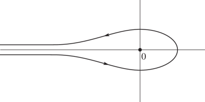
35: 5.9 Integral Representations

… ►

►►

Figure 5.9.1: $t$-plane. Contour for Hankel’s loop integral. Magnify

…

36: 31.10 Integral Equations and Representations

… ►

31.10.1 $$W(z)={\int }_C𝒦(z,t)w(t)\rho (t)dt$$

ⓘ

Defines:

$W(z)$: solution (locally)

Symbols:

$dx$: differential of $x$ , $\int$: integral, $z$: complex variable, $C$: contour, $\rho (t)$: weight function and $𝒦(z,t)$: kernel

Referenced by:

§31.10(i), §31.10(i)

Permalink:

http://dlmf.nist.gov/31.10.E1

Encodings:

pMML, png, TeX

See also:

Annotations for §31.10(i), §31.10 and Ch.31

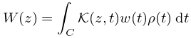
… ►For suitable choices of the branches of the $P$-symbols in (31.10.9) and the contour $C$, we can obtain both integral equations satisfied by Heun functions, as well as the integral representations of a distinct solution of Heun’s equation in terms of a Heun function (polynomial, path-multiplicative solution). … ►

31.10.12 $$W(z)={\int }_{C_1}{\int }_{C_2}𝒦(z;s,t)w(s)w(t)\rho (s,t)dsdt$$

ⓘ

Defines:

$W(z)$: solution (locally)

Symbols:

$dx$: differential of $x$ , $\int$: integral, $z$: complex variable, $C_1$, $C_2$: contours, $\rho (s,t)$: weight function, $𝒦(z;s,t)$: kernel and $w$

Permalink:

http://dlmf.nist.gov/31.10.E12

Encodings:

pMML, png, TeX

See also:

Annotations for §31.10(ii), §31.10 and Ch.31

…

37: 3.4 Differentiation

… ►

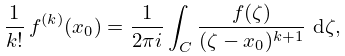
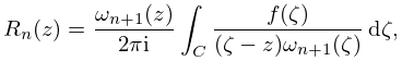
3.4.17 $$\frac{1}{k!}{f}^{(k)}(x_0)=\frac{1}{2\pi \mathrm{i}}{\int }_C\frac{f(\zeta )}{{(\zeta -x_0)}^{k+1}}d\zeta ,$$

ⓘ

Symbols:

$\pi$: the ratio of the circumference of a circle to its diameter, $dx$: differential of $x$ , $!$: factorial (as in $n!$), $\mathrm{i}$: imaginary unit, $\int$: integral and $C$: simple closed contour

Permalink:

http://dlmf.nist.gov/3.4.E17

Encodings:

pMML, png, TeX

See also:

Annotations for §3.4(ii), §3.4 and Ch.3

…

38: 15.6 Integral Representations

… ►In (15.6.2) the point $1/z$ lies outside the integration contour, $t^{b-1}$ and ${(t-1)}^{c-b-1}$ assume their principal values where the contour cuts the interval $(1,\mathrm{\infty })$, and ${(1-zt)}^a=1$ at $t=0$. ►In (15.6.3) the point $1/(z-1)$ lies outside the integration contour, the contour cuts the real axis between $t=-1$ and $0$, at which point $\mathrm{ph}t=\pi$ and $\mathrm{ph}\left(1+t\right)=0$. ►In (15.6.4) the point $1/z$ lies outside the integration contour, and at the point where the contour cuts the negative real axis $\mathrm{ph}t=\pi$ and $\mathrm{ph}\left(1-t\right)=0$. ►In (15.6.5) the integration contour starts and terminates at a point $A$ on the real axis between $0$ and $1$. …However, this reverses the direction of the integration contour, and in consequence (15.6.5) would need to be multiplied by $-1$. …

39: 3.3 Interpolation

… ►

3.3.6 $$R_n(z)=\frac{{\omega }_{n+1}(z)}{2\pi \mathrm{i}}{\int }_C\frac{f(\zeta )}{(\zeta -z){\omega }_{n+1}(\zeta )}d\zeta ,$$

ⓘ

Symbols:

$\pi$: the ratio of the circumference of a circle to its diameter, $dx$: differential of $x$ , $\mathrm{i}$: imaginary unit, $\int$: integral, $f(z)$: function, ${\omega }_{n+1}(z)$: nodal polynomial, $R_n(x)$: remainder and $C$: simple closed contour in $D$

A&S Ref:

25.2.5

Permalink:

http://dlmf.nist.gov/3.3.E6

Encodings:

pMML, png, TeX

See also:

Annotations for §3.3(i), §3.3 and Ch.3

… ►

3.3.37 $$\left[z_0,z_1,\mathrm{\dots },z_n\right]f=\frac{1}{2\pi \mathrm{i}}{\int }_C\frac{f(\zeta )}{{\omega }_{n+1}(\zeta )}d\zeta ,$$

ⓘ

Symbols:

$\pi$: the ratio of the circumference of a circle to its diameter, $dx$: differential of $x$ , $\left[z_0,z_1,\mathrm{\dots },z_n\right]f$: divided difference, $\mathrm{i}$: imaginary unit, $\int$: integral, $f(z)$: function, $C$: simple closed contour in $D$ , $z_k$: nodes of function and ${\omega }_{n+1}(z)$: nodal polynomial

Permalink:

http://dlmf.nist.gov/3.3.E37

Encodings:

pMML, png, TeX

See also:

Annotations for §3.3(iii), §3.3 and Ch.3

…

40: 36.15 Methods of Computation

… ►This can be carried out by direct numerical evaluation of canonical integrals along a finite segment of the real axis including all real critical points of $\mathrm{\Phi }$, with contributions from the contour outside this range approximated by the first terms of an asymptotic series associated with the endpoints. …