complete integrals

SearchAdvancedHelp

(0.007 seconds)

11—20 of 107 matching pages

11: 19.38 Approximations

… ►Minimax polynomial approximations (§3.11(i)) for $K\left(k\right)$ and $E\left(k\right)$ in terms of $m=k^2$ with can be found in Abramowitz and Stegun (1964, §17.3) with maximum absolute errors ranging from 4×10⁻⁵ to 2×10⁻⁸. Approximations of the same type for $K\left(k\right)$ and $E\left(k\right)$ for are given in Cody (1965a) with maximum absolute errors ranging from 4×10⁻⁵ to 4×10⁻¹⁸. … ►Approximations for Legendre’s complete or incomplete integrals of all three kinds, derived by Padé approximation of the square root in the integrand, are given in Luke (1968, 1970). …

12: 29.16 Asymptotic Expansions

… ►The approximations for Lamé polynomials hold uniformly on the rectangle $0\le \mathrm{\Re }z\le K$, $0\le \mathrm{\Im }z\le K^{\prime }$, when $nk$ and $n{k}^{\prime }$ assume large real values. …

13: 19.4 Derivatives and Differential Equations

… ►

${\displaystyle \frac{dK\left(k\right)}{dk}}={\displaystyle \frac{E\left(k\right)-k_{}^{\prime }{}_{}{}^{2}K\left(k\right)}{kk_{}^{\prime }{}_{}{}^2}},$

►

${\displaystyle \frac{d(E\left(k\right)-k_{}^{\prime }{}_{}{}^{2}K\left(k\right))}{dk}}=kK\left(k\right),$

►

${\displaystyle \frac{dE\left(k\right)}{dk}}={\displaystyle \frac{E\left(k\right)-K\left(k\right)}{k}},$

►

${\displaystyle \frac{d(E\left(k\right)-K\left(k\right))}{dk}}=-{\displaystyle \frac{kE\left(k\right)}{k_{}^{\prime }{}_{}{}^2}},$

… ►If $\varphi =\pi /2$, then these two equations become hypergeometric differential equations (15.10.1) for $K\left(k\right)$ and $E\left(k\right)$. …

14: 22.5 Special Values

… ►Table 22.5.1 gives the value of each of the 12 Jacobian elliptic functions, together with its $z$-derivative (or at a pole, the residue), for values of $z$ that are integer multiples of $K$, $\mathrm{i}{K}^{\prime }$. … ►

Table 22.5.1: Jacobian elliptic function values, together with derivatives or residues, for special values of the variable.

► ►►►

	$z$
	$0$	$K$	$K+\mathrm{i}{K}^{\prime }$	$\mathrm{i}{K}^{\prime }$	$2K$	$2K+2\mathrm{i}{K}^{\prime }$	$2\mathrm{i}{K}^{\prime }$
…

►

… ►

Table 22.5.2: Other special values of Jacobian elliptic functions.

► ►►►►

	$z$
	$\frac{1}{2}K$	$\frac{1}{2}(K+\mathrm{i}{K}^{\prime })$	$\frac{1}{2}\mathrm{i}{K}^{\prime }$
…
	$\frac{3}{2}K$	$\frac{3}{2}(K+\mathrm{i}{K}^{\prime })$	$\frac{3}{2}\mathrm{i}{K}^{\prime }$
…

►

… ►Expansions for $K,K^{\prime }$ as $k\to 0$ or $1$ are given in §§19.5, 19.12. …

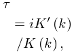
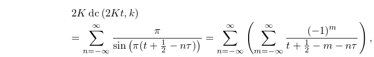
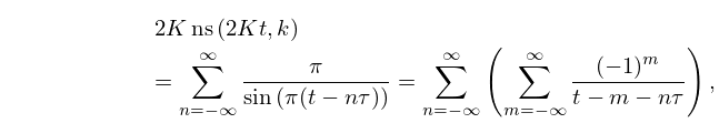
15: 22.12 Expansions in Other Trigonometric Series and Doubly-Infinite Partial Fractions: Eisenstein Series

… ►

22.12.1 $$\tau =\mathrm{i}{K}^{\prime }\left(k\right)/K\left(k\right),$$

ⓘ

Symbols:

$K^{\prime }\left(k\right)$: Legendre’s complementary complete elliptic integral of the first kind, $K\left(k\right)$: Legendre’s complete elliptic integral of the first kind, $\mathrm{i}$: imaginary unit, $k$: modulus and $\tau$: ratio

Permalink:

http://dlmf.nist.gov/22.12.E1

Encodings:

pMML, png, TeX

See also:

Annotations for §22.12 and Ch.22

►

22.12.2 $$2Kk\mathrm{sn}(2Kt,k)=\sum _{n=-\mathrm{\infty }}^{\mathrm{\infty }}\frac{\pi }{\sin \left(\pi (t-(n+\frac{1}{2})\tau )\right)}=\sum _{n=-\mathrm{\infty }}^{\mathrm{\infty }}\left(\sum _{m=-\mathrm{\infty }}^{\mathrm{\infty }}\frac{{(-1)}^m}{t-m-(n+\frac{1}{2})\tau }\right),$$

ⓘ

Symbols:

$\mathrm{sn}(z,k)$: Jacobian elliptic function, $\pi$: the ratio of the circumference of a circle to its diameter, $K\left(k\right)$: Legendre’s complete elliptic integral of the first kind, $\sin z$: sine function, $k$: modulus and $\tau$: ratio

Referenced by:

§22.12, §22.12

Permalink:

http://dlmf.nist.gov/22.12.E2

Encodings:

pMML, png, TeX

See also:

Annotations for §22.12 and Ch.22

… ►

22.12.8 $$2K\mathrm{dc}(2Kt,k)=\sum _{n=-\mathrm{\infty }}^{\mathrm{\infty }}\frac{\pi }{\sin \left(\pi (t+\frac{1}{2}-n\tau )\right)}=\sum _{n=-\mathrm{\infty }}^{\mathrm{\infty }}\left(\sum _{m=-\mathrm{\infty }}^{\mathrm{\infty }}\frac{{(-1)}^m}{t+\frac{1}{2}-m-n\tau }\right),$$

ⓘ

Symbols:

$\mathrm{dc}(z,k)$: Jacobian elliptic function, $\pi$: the ratio of the circumference of a circle to its diameter, $K\left(k\right)$: Legendre’s complete elliptic integral of the first kind, $\sin z$: sine function, $k$: modulus and $\tau$: ratio

Permalink:

http://dlmf.nist.gov/22.12.E8

Encodings:

pMML, png, TeX

See also:

Annotations for §22.12 and Ch.22

… ►

22.12.11 $$2K\mathrm{ns}(2Kt,k)=\sum _{n=-\mathrm{\infty }}^{\mathrm{\infty }}\frac{\pi }{\sin \left(\pi (t-n\tau )\right)}=\sum _{n=-\mathrm{\infty }}^{\mathrm{\infty }}\left(\sum _{m=-\mathrm{\infty }}^{\mathrm{\infty }}\frac{{(-1)}^m}{t-m-n\tau }\right),$$

ⓘ

Symbols:

$\mathrm{ns}(z,k)$: Jacobian elliptic function, $\pi$: the ratio of the circumference of a circle to its diameter, $K\left(k\right)$: Legendre’s complete elliptic integral of the first kind, $\sin z$: sine function, $k$: modulus and $\tau$: ratio

Permalink:

http://dlmf.nist.gov/22.12.E11

Encodings:

pMML, png, TeX

See also:

Annotations for §22.12 and Ch.22

►

22.12.12 $$2K\mathrm{ds}(2Kt,k)=\sum _{n=-\mathrm{\infty }}^{\mathrm{\infty }}\frac{{(-1)}^n\pi }{\sin \left(\pi (t-n\tau )\right)}=\sum _{n=-\mathrm{\infty }}^{\mathrm{\infty }}\left(\sum _{m=-\mathrm{\infty }}^{\mathrm{\infty }}\frac{{(-1)}^{m+n}}{t-m-n\tau }\right),$$

ⓘ

Symbols:

$\mathrm{ds}(z,k)$: Jacobian elliptic function, $\pi$: the ratio of the circumference of a circle to its diameter, $K\left(k\right)$: Legendre’s complete elliptic integral of the first kind, $\sin z$: sine function, $k$: modulus and $\tau$: ratio

Permalink:

http://dlmf.nist.gov/22.12.E12

Encodings:

pMML, png, TeX

See also:

Annotations for §22.12 and Ch.22

…

16: 19.6 Special Cases

… ►

$K\left(0\right)=E\left(0\right)=K^{\prime }\left(1\right)=E^{\prime }\left(1\right)=\frac{1}{2}\pi ,$

►

$K\left(1\right)=K^{\prime }\left(0\right)=\mathrm{\infty },$

►

$E\left(1\right)=E^{\prime }\left(0\right)=1.$

… ►

$$\mathrm{\Pi }({\alpha }^2,k)\to K\left(k\right)-\left(E\left(k\right)/k_{}^{\prime }{}_{}{}^2\right),$$ ${\alpha }^2\to 1+$,

… ►Exact values of $K\left(k\right)$ and $E\left(k\right)$ for various special values of $k$ are given in Byrd and Friedman (1971, 111.10 and 111.11) and Cooper et al. (2006). …

17: 22.1 Special Notation

… ► ►►►►

$x,y$	real variables.
…
$K$, $K^{\prime }$	$K\left(k\right)$, $K^{\prime }\left(k\right)=K\left(k^{\prime }\right)$ (complete elliptic integrals of the first kind (§19.2(ii))).
…
$\tau$	$\mathrm{i}{K}^{\prime }/K$.

…

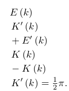
18: 19.7 Connection Formulas

… ►

19.7.1 $$E\left(k\right)K^{\prime }\left(k\right)+E^{\prime }\left(k\right)K\left(k\right)-K\left(k\right)K^{\prime }\left(k\right)=\frac{1}{2}\pi .$$

ⓘ

Symbols:

$\pi$: the ratio of the circumference of a circle to its diameter, $K^{\prime }\left(k\right)$: Legendre’s complementary complete elliptic integral of the first kind, $E^{\prime }\left(k\right)$: Legendre’s complementary complete elliptic integral of the second kind, $K\left(k\right)$: Legendre’s complete elliptic integral of the first kind, $E\left(k\right)$: Legendre’s complete elliptic integral of the second kind and $k$: real or complex modulus

Referenced by:

§19.21(i), §19.35(i), §19.7(i)

Permalink:

http://dlmf.nist.gov/19.7.E1

Encodings:

pMML, png, TeX

See also:

Annotations for §19.7(i), §19.7(i), §19.7 and Ch.19

… ►

$K\left(\mathrm{i}k/k^{\prime }\right)=k^{\prime }K\left(k\right),$

►

$K\left(-\mathrm{i}{k}^{\prime }/k\right)=kK\left(k^{\prime }\right),$

… ►

$$K\left(1/k\right)=k(K\left(k\right)\mp \mathrm{i}K\left(k^{\prime }\right)),$$

►

$$K\left(1/k^{\prime }\right)=k^{\prime }(K\left(k^{\prime }\right)\pm \mathrm{i}K\left(k\right)),$$

…

19: 19.13 Integrals of Elliptic Integrals

… ►For definite and indefinite integrals of complete elliptic integrals see Byrd and Friedman (1971, pp. 610–612, 615), Prudnikov et al. (1990, §§1.11, 2.16), Glasser (1976), Bushell (1987), and Cvijović and Klinowski (1999). … ►For direct and inverse Laplace transforms for the complete elliptic integrals $K\left(k\right)$, $E\left(k\right)$, and $D\left(k\right)$ see Prudnikov et al. (1992a, §3.31) and Prudnikov et al. (1992b, §§3.29 and 4.3.33), respectively.

20: 19.37 Tables

… ►

§19.37(ii) Legendre’s Complete Integrals

►

Functions $K\left(k\right)$ and $E\left(k\right)$

►Tabulated for $k^2=0(.01)1$ to 6D by Byrd and Friedman (1971), to 15D for $K\left(k\right)$ and 9D for $E\left(k\right)$ by Abramowitz and Stegun (1964, Chapter 17), and to 10D by Fettis and Caslin (1964). … ►

Functions $K\left(k\right)$, $K^{\prime }\left(k\right)$, and $\mathrm{i}{K}^{\prime }\left(k\right)/K\left(k\right)$

… ►

Function $\exp \left(-\pi K^{\prime }\left(k\right)/K\left(k\right)\right)(=q(k))$

…