comparison with Gauss quadrature

SearchAdvancedHelp

(0.001 seconds)

21—30 of 151 matching pages

21: Bibliography I

… ►

Highly Oscillatory Quadrature: The Story So Far. In Numerical Mathematics and Advanced Applications, A. Bermudez de Castro and others (Eds.), pp. 97–118.

ⓘ

Notes:

Proceedings of ENuMath, Santiago de Compostela (2005)

External Links:

ISBN 3-540-34287-7, MathReview, ZentralBlatt

Referenced by:

§3.5(vii).

Encodings:

BibTeX

… ►

From Gauss to Painlevé: A Modern Theory of Special Functions. Aspects of Mathematics E, Vol. 16, Friedr. Vieweg & Sohn, Braunschweig, Germany.

ⓘ

External Links:

ISBN 3-528-06355-6, MathReview (Takeshi Sasaki), ZentralBlatt

Referenced by:

§32.2(vi), §32.7(vii).

Encodings:

BibTeX

22: 18.2 General Orthogonal Polynomials

… ►For usage of the zeros of an OP in Gauss quadrature see §3.5(v). … ►resulting in $p_n^{(0)}(x)=p_{n-1}^{(1)}(x)$, by simple comparison of the two recursions. …

23: 15.5 Derivatives and Contiguous Functions

… ►The six functions $F(a\pm 1,b;c;z)$, $F(a,b\pm 1;c;z)$, $F(a,b;c\pm 1;z)$ are said to be contiguous to $F(a,b;c;z)$. ►

15.5.11 $$(c-a)F(a-1,b;c;z)+\left(2a-c+(b-a)z\right)F(a,b;c;z)+a(z-1)F(a+1,b;c;z)=0,$$

ⓘ

Symbols:

$F(a,b;c;z)$ or $F(\genfrac{}{}{0pt}{}{a,b}{c};z)$: $={}_2{}^{}F_1^{}(a,b;c;z)$ Gauss’ hypergeometric function, $z$: complex variable, $a$: real or complex parameter, $b$: real or complex parameter and $c$: real or complex parameter

Referenced by:

§15.4(i), §15.5(ii)

Permalink:

http://dlmf.nist.gov/15.5.E11

Encodings:

pMML, png, TeX

See also:

Annotations for §15.5(ii), §15.5 and Ch.15

►

15.5.12 $$(b-a)F(a,b;c;z)+aF(a+1,b;c;z)-bF(a,b+1;c;z)=0,$$

ⓘ

Symbols:

$F(a,b;c;z)$ or $F(\genfrac{}{}{0pt}{}{a,b}{c};z)$: $={}_2{}^{}F_1^{}(a,b;c;z)$ Gauss’ hypergeometric function, $z$: complex variable, $a$: real or complex parameter, $b$: real or complex parameter and $c$: real or complex parameter

Permalink:

http://dlmf.nist.gov/15.5.E12

Encodings:

pMML, png, TeX

See also:

Annotations for §15.5(ii), §15.5 and Ch.15

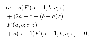
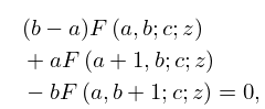
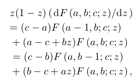
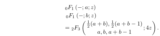
… ►By repeated applications of (15.5.11)–(15.5.18) any function $F(a+k,b+\mathrm{\ell };c+m;z)$, in which $k,\mathrm{\ell },m$ are integers, can be expressed as a linear combination of $F(a,b;c;z)$ and any one of its contiguous functions, with coefficients that are rational functions of $a,b,c$, and $z$. … ►

15.5.20 $$z(1-z)\left(dF(a,b;c;z)/dz\right)=(c-a)F(a-1,b;c;z)+(a-c+bz)F(a,b;c;z)=(c-b)F(a,b-1;c;z)+(b-c+az)F(a,b;c;z),$$

ⓘ

Symbols:

$F(a,b;c;z)$ or $F(\genfrac{}{}{0pt}{}{a,b}{c};z)$: $={}_2{}^{}F_1^{}(a,b;c;z)$ Gauss’ hypergeometric function, $\frac{df}{dx}$: derivative of $f$ with respect to $x$ , $z$: complex variable, $a$: real or complex parameter, $b$: real or complex parameter and $c$: real or complex parameter

Permalink:

http://dlmf.nist.gov/15.5.E20

Encodings:

pMML, png, TeX

See also:

Annotations for §15.5(ii), §15.5 and Ch.15

…

24: Bibliography S

… ►

A Gaussian quadrature for the calculation of generalized Fermi-Dirac integrals. Comput. Phys. Comm. 66 (2-3), pp. 271–275.

ⓘ

External Links:

ISSN 0010-4655, Document, MathReview, ZentralBlatt

Referenced by:

§25.18(i).

Encodings:

BibTeX

… ►

Sturm oscillation and comparison theorems. In Sturm-Liouville theory, pp. 29–43.

ⓘ

External Links:

Document, Link, MathReview Entry

Referenced by:

§18.36(vi), §18.39(i).

Encodings:

BibTeX

… ►

Gaussian Quadrature Formulas. Prentice-Hall Inc., Englewood Cliffs, N.J..

ⓘ

External Links:

MathReview (P. C. Hammer), ZentralBlatt

Referenced by:

§3.5(v).

Encodings:

BibTeX

…

25: 2.4 Contour Integrals

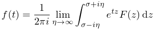
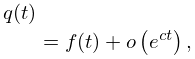
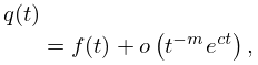
… ►For large $t$, the asymptotic expansion of $q(t)$ may be obtained from (2.4.3) by Haar’s method. This depends on the availability of a comparison function $F(z)$ for $Q(z)$ that has an inverse transform ►

2.4.6 $$f(t)=\frac{1}{2\pi \mathrm{i}}\underset{\eta \to \mathrm{\infty }}{lim}{\int }_{\sigma -\mathrm{i}\eta }^{\sigma +\mathrm{i}\eta }{\mathrm{e}}^{tz}F(z)dz$$

ⓘ

Symbols:

$\pi$: the ratio of the circumference of a circle to its diameter, $dx$: differential of $x$ , $\mathrm{e}$: base of natural logarithm, $\mathrm{i}$: imaginary unit, $\int$: integral, $\sigma$: constant, $F(z)$: comparison function and $f(x)$: inverse transform of comparison function

Permalink:

http://dlmf.nist.gov/2.4.E6

Encodings:

pMML, png, TeX

See also:

Annotations for §2.4(ii), §2.4 and Ch.2

… ►

2.4.7 $$q(t)-f(t)=\frac{{\mathrm{e}}^{\sigma t}}{2\pi }\underset{\eta \to \mathrm{\infty }}{lim}{\int }_{-\eta }^{\eta }{\mathrm{e}}^{\mathrm{i}t\tau }(Q(\sigma +\mathrm{i}\tau )-F(\sigma +\mathrm{i}\tau ))d\tau .$$

ⓘ

Symbols:

$\pi$: the ratio of the circumference of a circle to its diameter, $dx$: differential of $x$ , $\mathrm{e}$: base of natural logarithm, $\mathrm{i}$: imaginary unit, $\int$: integral, $q(t)$: analytic function, $Q(z)$: Laplace transform of $q(t)$ , $\sigma$: constant, $F(z)$: comparison function and $f(x)$: inverse transform of comparison function

Permalink:

http://dlmf.nist.gov/2.4.E7

Encodings:

pMML, png, TeX

See also:

Annotations for §2.4(ii), §2.4 and Ch.2

… ►

2.4.8 $$q(t)=f(t)+o\left({\mathrm{e}}^{ct}\right),$$ $t\to +\mathrm{\infty }$.

ⓘ

Symbols:

$\mathrm{e}$: base of natural logarithm, $o\left(x\right)$: order less than, $q(t)$: analytic function, $c$: real constant and $f(x)$: inverse transform of comparison function

Permalink:

http://dlmf.nist.gov/2.4.E8

Encodings:

pMML, png, TeX

See also:

Annotations for §2.4(ii), §2.4 and Ch.2

… ►

2.4.9 $$q(t)=f(t)+o\left(t^{-m}{\mathrm{e}}^{ct}\right),$$ $t\to +\mathrm{\infty }$.

ⓘ

Symbols:

$\mathrm{e}$: base of natural logarithm, $o\left(x\right)$: order less than, $q(t)$: analytic function, $c$: real constant and $f(x)$: inverse transform of comparison function

Permalink:

http://dlmf.nist.gov/2.4.E9

Encodings:

pMML, png, TeX

See also:

Annotations for §2.4(ii), §2.4 and Ch.2

…

26: 15.3 Graphics

… ►

►►

Figure 15.3.1: $F(\frac{4}{3},\frac{9}{16};\frac{14}{5};x),-100\le x\le 1$. Magnify

►

►►

Figure 15.3.2: $F(5,-10;1;x),-0.023\le x\le 1$. Magnify

►

►►

Figure 15.3.3: $F(1,-10;10;x),-3\le x\le 1$. Magnify

►

►►

Figure 15.3.4: $F(5,10;1;x),-1\le x\le 0.022$. Magnify

… ►

►

►

Figure 15.3.5: $F(\frac{4}{3},\frac{9}{16};\frac{14}{5};x+\mathrm{i}y),0\le x\le 2,-0.5\le y\le 0.5$. … Magnify 3D Help

…

27: 16.12 Products

… ►

16.12.1 $${}_0{}^{}F_1^{}(-;a;z){}_0{}^{}F_1^{}(-;b;z)={}_2{}^{}F_3^{}(\genfrac{}{}{0pt}{}{\frac{1}{2}(a+b),\frac{1}{2}(a+b-1)}{a,b,a+b-1};4z).$$

ⓘ

Symbols:

${}_p{}^{}F_q^{}(a_1,\mathrm{\dots },a_p;b_1,\mathrm{\dots },b_q;z)$ or ${}_p{}^{}F_q^{}(\genfrac{}{}{0pt}{}{a_1,\mathrm{\dots },a_p}{b_1,\mathrm{\dots },b_q};z)$: alternatively ${}_p{}^{}F_q^{}(𝐚;𝐛;z)$ or ${}_p{}^{}F_q^{}(\genfrac{}{}{0pt}{}{𝐚}{𝐛};z)$
generalized hypergeometric function, $z$: complex variable, $a,a_1,\mathrm{\dots },a_p$: real or complex parameters and $b,b_1,\mathrm{\dots },b_q$: real or complex parameters

Referenced by:

(10.8.3), §10.8, §10.8, §16.12, Erratum (V1.0.17) for Section 10.8

Permalink:

http://dlmf.nist.gov/16.12.E1

Encodings:

pMML, png, TeX

See also:

Annotations for §16.12 and Ch.16

… ►

16.12.2 $${\left({}_2{}^{}F_1^{}(\genfrac{}{}{0pt}{}{a,b}{a+b+\frac{1}{2}};z)\right)}^2={}_3{}^{}F_2^{}(\genfrac{}{}{0pt}{}{2a,2b,a+b}{a+b+\frac{1}{2},2a+2b};z).$$

ⓘ

Symbols:

${}_2{}^{}F_1^{}(a,b;c;z)$: $=F(a,b;c;z)$ notation for Gauss’ hypergeometric function, ${}_p{}^{}F_q^{}(a_1,\mathrm{\dots },a_p;b_1,\mathrm{\dots },b_q;z)$ or ${}_p{}^{}F_q^{}(\genfrac{}{}{0pt}{}{a_1,\mathrm{\dots },a_p}{b_1,\mathrm{\dots },b_q};z)$: alternatively ${}_p{}^{}F_q^{}(𝐚;𝐛;z)$ or ${}_p{}^{}F_q^{}(\genfrac{}{}{0pt}{}{𝐚}{𝐛};z)$
generalized hypergeometric function, $z$: complex variable, $a,a_1,\mathrm{\dots },a_p$: real or complex parameters and $b,b_1,\mathrm{\dots },b_q$: real or complex parameters

Referenced by:

§16.12, §17.9(iii), Erratum (V1.1.12) for Subsection 17.9(iii)

Permalink:

http://dlmf.nist.gov/16.12.E2

Encodings:

pMML, png, TeX

See also:

Annotations for §16.12 and Ch.16

… ►

16.12.3 $${\left({}_2{}^{}F_1^{}(\genfrac{}{}{0pt}{}{a,b}{c};z)\right)}^2=\sum _{k=0}^{\mathrm{\infty }}\frac{{\left(2a\right)}_k{\left(2b\right)}_k{\left(c-\frac{1}{2}\right)}_k}{{\left(c\right)}_k{\left(2c-1\right)}_{k}k!}{}_4{}^{}F_3^{}(\genfrac{}{}{0pt}{}{-\frac{1}{2}k,\frac{1}{2}(1-k),a+b-c+\frac{1}{2},\frac{1}{2}}{a+\frac{1}{2},b+\frac{1}{2},\frac{3}{2}-k-c};1)z^k,$$ .

ⓘ

Symbols:

${}_2{}^{}F_1^{}(a,b;c;z)$: $=F(a,b;c;z)$ notation for Gauss’ hypergeometric function, ${}_p{}^{}F_q^{}(a_1,\mathrm{\dots },a_p;b_1,\mathrm{\dots },b_q;z)$ or ${}_p{}^{}F_q^{}(\genfrac{}{}{0pt}{}{a_1,\mathrm{\dots },a_p}{b_1,\mathrm{\dots },b_q};z)$: alternatively ${}_p{}^{}F_q^{}(𝐚;𝐛;z)$ or ${}_p{}^{}F_q^{}(\genfrac{}{}{0pt}{}{𝐚}{𝐛};z)$
generalized hypergeometric function, ${\left(a\right)}_n$: Pochhammer’s symbol (or shifted factorial), $!$: factorial (as in $n!$), $z$: complex variable, $a,a_1,\mathrm{\dots },a_p$: real or complex parameters and $b,b_1,\mathrm{\dots },b_q$: real or complex parameters

Referenced by:

§16.12

Permalink:

http://dlmf.nist.gov/16.12.E3

Encodings:

pMML, png, TeX

See also:

Annotations for §16.12 and Ch.16

…

28: 15.4 Special Cases

… ►

15.4.1 $$F(1,1;2;z)=-z^{-1}\ln \left(1-z\right),$$

ⓘ

Symbols:

$F(a,b;c;z)$ or $F(\genfrac{}{}{0pt}{}{a,b}{c};z)$: $={}_2{}^{}F_1^{}(a,b;c;z)$ Gauss’ hypergeometric function, $\ln z$: principal branch of logarithm function and $z$: complex variable

Referenced by:

§15.4(i)

Permalink:

http://dlmf.nist.gov/15.4.E1

Encodings:

pMML, png, TeX

See also:

Annotations for §15.4(i), §15.4 and Ch.15

►

15.4.2 $$F(\frac{1}{2},1;\frac{3}{2};z^2)=\frac{1}{2z}\ln \left(\frac{1+z}{1-z}\right),$$

ⓘ

Symbols:

$F(a,b;c;z)$ or $F(\genfrac{}{}{0pt}{}{a,b}{c};z)$: $={}_2{}^{}F_1^{}(a,b;c;z)$ Gauss’ hypergeometric function, $\ln z$: principal branch of logarithm function and $z$: complex variable

Permalink:

http://dlmf.nist.gov/15.4.E2

Encodings:

pMML, png, TeX

See also:

Annotations for §15.4(i), §15.4 and Ch.15

►

15.4.3 $$F(\frac{1}{2},1;\frac{3}{2};-z^2)=z^{-1}\arctan z,$$

ⓘ

Symbols:

$F(a,b;c;z)$ or $F(\genfrac{}{}{0pt}{}{a,b}{c};z)$: $={}_2{}^{}F_1^{}(a,b;c;z)$ Gauss’ hypergeometric function, $\arctan z$: arctangent function and $z$: complex variable

Permalink:

http://dlmf.nist.gov/15.4.E3

Encodings:

pMML, png, TeX

See also:

Annotations for §15.4(i), §15.4 and Ch.15

… ►

$$F(a,b;a;z)={(1-z)}^{-b},$$

►

$$F(a,b;b;z)={(1-z)}^{-a},$$

…

29: 5.21 Methods of Computation

… ►Another approach is to apply numerical quadrature (§3.5) to the integral (5.9.2), using paths of steepest descent for the contour. …

30: 15.1 Special Notation

… ►

15.1.1 $${}_2{}^{}F_1^{}(a,b;c;z)=F(a,b;c;z)=F(\genfrac{}{}{0pt}{}{a,b}{c};z),$$

ⓘ

Symbols:

$F(a,b;c;z)$ or $F(\genfrac{}{}{0pt}{}{a,b}{c};z)$: $={}_2{}^{}F_1^{}(a,b;c;z)$ Gauss’ hypergeometric function, ${}_2{}^{}F_1^{}(a,b;c;z)$: $=F(a,b;c;z)$ notation for Gauss’ hypergeometric function, $z$: complex variable, $a$: real or complex parameter, $b$: real or complex parameter and $c$: real or complex parameter

Permalink:

http://dlmf.nist.gov/15.1.E1

Encodings:

pMML, png, TeX

See also:

Annotations for §15.1 and Ch.15

… ►

15.1.2 $$\frac{F(a,b;c;z)}{\mathrm{\Gamma }\left(c\right)}=𝐅(a,b;c;z)=𝐅(\genfrac{}{}{0pt}{}{a,b}{c};z)={}_2{}^{}𝐅_1^{}(a,b;c;z),$$

ⓘ

Symbols:

$\mathrm{\Gamma }\left(z\right)$: gamma function, $F(a,b;c;z)$ or $F(\genfrac{}{}{0pt}{}{a,b}{c};z)$: $={}_2{}^{}F_1^{}(a,b;c;z)$ Gauss’ hypergeometric function, ${}_p{}^{}𝐅_q^{}(𝐚;𝐛;z)$ or ${}_p{}^{}𝐅_q^{}(\genfrac{}{}{0pt}{}{𝐚}{𝐛};z)$: scaled (or Olver’s) generalized hypergeometric function, $𝐅(a,b;c;z)$ or $𝐅(\genfrac{}{}{0pt}{}{a,b}{c};z)$: $={}_2{}^{}𝐅_1^{}(a,b;c;z)$ Olver’s hypergeometric function, $z$: complex variable, $a$: real or complex parameter, $b$: real or complex parameter and $c$: real or complex parameter

Permalink:

http://dlmf.nist.gov/15.1.E2

Encodings:

pMML, png, TeX

See also:

Annotations for §15.1 and Ch.15

…