closed
(0.001 seconds)
31—40 of 151 matching pages
31: 26.15 Permutations: Matrix Notation
32: 1.5 Calculus of Two or More Variables
…
►Suppose that are finite, is finite or , and , are continuous on the partly-closed rectangle or infinite strip .
…for all and all .
…
►Let be defined on a closed rectangle .
For
…let denote any point in the rectangle , , .
…
33: 1.10 Functions of a Complex Variable
…
►Suppose the subarc , is contained in a domain , .
…
►Let be a simple closed contour consisting of a segment of the real axis and a contour in the upper half-plane joining the ends of .
…
►Let be a domain and be a closed finite segment of the real axis.
Assume that for each , is an analytic function of in , and also that is a continuous function of both variables.
…
►For each , is analytic in ; is a continuous function of both variables when and ; the integral (1.10.18) converges at , and this convergence is uniform with respect to in every compact subset of .
…
34: 1.8 Fourier Series
…
►where is square-integrable on and are given by (1.8.2), (1.8.4).
…
►For piecewise continuous on and real ,
…
►If and are the Fourier coefficients of a piecewise continuous function on , then
…
►Suppose that is continuous and of bounded variation on .
Suppose also that is integrable on and as .
…
35: 1.18 Linear Second Order Differential Operators and Eigenfunction Expansions
…
►Let or or or be a (possibly infinite, or semi-infinite) interval in .
…
►Consider the second order differential operator acting on real functions of in the finite interval
…
►The nature of these extensions for unbounded intervals such as , and unbounded operators on them, are the subject of §1.18(ix).
…
►
Example 1: Bessel–Hankel Transform,
… ►For piecewise continuously differentiable on …36: 3.5 Quadrature
…
►where , , and .
…
►Let and .
…
►If , then the remainder in (3.5.2) can be expanded in the form
…
►is computed with on the interval .
…
►Rules of closed type include the Newton–Cotes formulas such as the trapezoidal rules and Simpson’s rule.
…
37: 14.21 Definitions and Basic Properties
…
►When is complex , , and are defined by (14.3.6)–(14.3.10) with replaced by : the principal branches are obtained by taking the principal values of all the multivalued functions appearing in these representations when , and by continuity elsewhere in the -plane with a cut along the interval ; compare §4.2(i).
…
►Many of the properties stated in preceding sections extend immediately from the -interval to the cut -plane .
…
38: 25.12 Polylogarithms
…
►The principal branch has a cut along the interval and agrees with (25.12.1) when ; see also §4.2(i).
…
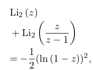
►
25.12.3
.
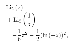
►
25.12.4
.
…
39: 1.13 Differential Equations
…
►
§1.13(vii) Closed-Form Solutions
… ►on a finite interval , this is then a regular Sturm-Liouville system. … ►Equation (1.13.26) with may be transformed to the Liouville normal form ►
1.13.29
…
►As the interval is mapped, one-to-one, onto by the above definition of , the integrand being positive, the inverse of this same transformation allows to be calculated from in (1.13.31), and .
…
40: 21.1 Special Notation
…
►
►
…
| positive integers. | |
| … | |
| -dimensional vectors, with all elements in , unless stated otherwise. | |
| … | |
| intersection index of and , two cycles lying on a closed surface. if and do not intersect. Otherwise gets an additive contribution from every intersection point. This contribution is if the basis of the tangent vectors of the and cycles (§21.7(i)) at the point of intersection is positively oriented; otherwise it is . | |
| … | |
