closed

SearchAdvancedHelp

(0.001 seconds)

11—20 of 151 matching pages

11: 8.15 Sums

… ►

8.15.2 $$a\sum _{k=1}^{\mathrm{\infty }}\left(\frac{{\mathrm{e}}^{2\pi \mathrm{i}k(z+h)}}{{\left(2\pi \mathrm{i}k\right)}^{a+1}}\mathrm{\Gamma }(a,2\pi \mathrm{i}kz)+\frac{{\mathrm{e}}^{-2\pi \mathrm{i}k(z+h)}}{{\left(-2\pi \mathrm{i}k\right)}^{a+1}}\mathrm{\Gamma }(a,-2\pi \mathrm{i}kz)\right)=\zeta (-a,z+h)+\frac{z^{a+1}}{a+1}+\left(h-\frac{1}{2}\right)z^a,$$ $h\in [0,1]$.

ⓘ

Symbols:

$\zeta (s,a)$: Hurwitz zeta function, $\pi$: the ratio of the circumference of a circle to its diameter, $[a,b]$: closed interval, $\in$: element of, $\mathrm{e}$: base of natural logarithm, $\mathrm{i}$: imaginary unit, $\mathrm{\Gamma }(a,z)$: incomplete gamma function, $z$: complex variable, $a$: parameter and $k$: nonnegative integer

Proof sketch:

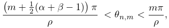
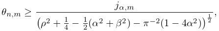
Start with and $z>0$. For $\mathrm{\Gamma }(a,\pm 2\pi \mathrm{i}kz)$ take integral representation (8.2.2) and use the substitution $t=\pm 2\pi \mathrm{i}kz(1+\tau )$. The sum and the integral can be interchanged, and the sum can be evaluated via (4.6.1). Use integration by parts. This will result in $\left(h-\frac{1}{2}\right)z^a$ plus two integrals with infinitely many poles. The residue theorem (§1.10(iv)) will give us an infinite series which can be identified via (25.11.1). For other values of $a$ and $z$ use analytic continuation.

Referenced by:

§25.11(x), §25.11(x), §8.15, Erratum (V1.1.3) for Additions

Permalink:

http://dlmf.nist.gov/8.15.E2

Encodings:

pMML, png, TeX

Addition (effective with 1.1.3):

This equation was added.

See also:

Annotations for §8.15 and Ch.8

…

12: 18.24 Hahn Class: Asymptotic Approximations

… ►With $\mu =N/n$ and $x$ fixed, Qiu and Wong (2004) gives an asymptotic expansion for $K_n(x;p,N)$ as $n\to \mathrm{\infty }$, that holds uniformly for $\mu \in [1,\mathrm{\infty })$. … ►Taken together, these expansions are uniformly valid for and for $a$ in unbounded intervals—each of which contains $[0,(1-\delta )n]$, where $\delta$ again denotes an arbitrary small positive constant. … ►These approximations are in terms of Laguerre polynomials and hold uniformly for $\mathrm{ph}\left(x+i\lambda \right)\in [0,\pi ]$. …

13: 3.11 Approximation Techniques

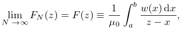
… ►Let $f(x)$ be continuous on a closed interval $[a,b]$. … ►If $f$ is continuously differentiable on $[-1,1]$, then with … ►For general intervals $[a,b]$ we rescale: … ►Let $f$ be continuous on a closed interval $[a,b]$ and $w$ be a continuous nonvanishing function on $[a,b]$: $w$ is called a weight function. …of type $[k,\mathrm{\ell }]$ to $f$ on $[a,b]$ minimizes the maximum value of $\left|{ϵ}_{k,\mathrm{\ell }}(x)\right|$ on $[a,b]$, where …

14: 18.16 Zeros

… ►

18.16.2 $${\theta }_{n,m}^{(-\frac{1}{2},\frac{1}{2})}=\frac{(m-\frac{1}{2})\pi }{n+\frac{1}{2}}\le {\theta }_{n,m}^{(\alpha ,\beta )}\le \frac{m\pi }{n+\frac{1}{2}}={\theta }_{n,m}^{(\frac{1}{2},-\frac{1}{2})},$$ $\alpha ,\beta \in [-\frac{1}{2},\frac{1}{2}]$,

ⓘ

Symbols:

$\pi$: the ratio of the circumference of a circle to its diameter, $[a,b]$: closed interval, $\in$: element of, $(a,b)$: open interval, $m$: nonnegative integer, $n$: nonnegative integer and ${\theta }_{n,m}$: zeros

Referenced by:

§18.16(iii), Erratum (V1.2.0) for Equations (18.16.2), (18.16.3)

Permalink:

http://dlmf.nist.gov/18.16.E2

Encodings:

pMML, png, TeX

See also:

Annotations for §18.16(ii), §18.16(ii), §18.16 and Ch.18

►

18.16.3 $${\theta }_{n,m}^{(-\frac{1}{2},-\frac{1}{2})}=\frac{(m-\frac{1}{2})\pi }{n}\le {\theta }_{n,m}^{(\alpha ,\alpha )}\le \frac{m\pi }{n+1}={\theta }_{n,m}^{(\frac{1}{2},\frac{1}{2})},$$ $\alpha \in [-\frac{1}{2},\frac{1}{2}]$, $m=1,2,\mathrm{\dots },\lfloor \frac{1}{2}n\rfloor$.

ⓘ

Symbols:

$\pi$: the ratio of the circumference of a circle to its diameter, $[a,b]$: closed interval, $\in$: element of, $\lfloor x\rfloor$: floor of $x$ , $(a,b)$: open interval, $m$: nonnegative integer, $n$: nonnegative integer and ${\theta }_{n,m}$: zeros

Referenced by:

§18.16(iii), Erratum (V1.2.0) for Equations (18.16.2), (18.16.3)

Permalink:

http://dlmf.nist.gov/18.16.E3

Encodings:

pMML, png, TeX

See also:

Annotations for §18.16(ii), §18.16(ii), §18.16 and Ch.18

… ►

18.16.4 $\alpha ,\beta \in [-\frac{1}{2},\frac{1}{2}]$,

ⓘ

Symbols:

$\pi$: the ratio of the circumference of a circle to its diameter, $[a,b]$: closed interval, $\in$: element of, $m$: nonnegative integer, $n$: nonnegative integer, $\rho$ and ${\theta }_{n,m}$: zeros

Permalink:

http://dlmf.nist.gov/18.16.E4

Encodings:

pMML, png, TeX

See also:

Annotations for §18.16(ii), §18.16(ii), §18.16 and Ch.18

… ►

18.16.6 $${\theta }_{n,m}\le \frac{j_{\alpha ,m}}{{\left({\rho }^2+\frac{1}{12}\left(1-{\alpha }^2-3{\beta }^2\right)\right)}^{\frac{1}{2}}},$$ $\alpha ,\beta \in [-\frac{1}{2},\frac{1}{2}]$,

ⓘ

Symbols:

$[a,b]$: closed interval, $\in$: element of, $m$: nonnegative integer, $n$: nonnegative integer, $\rho$ and ${\theta }_{n,m}$: zeros

Referenced by:

§18.16(ii)

Permalink:

http://dlmf.nist.gov/18.16.E6

Encodings:

pMML, png, TeX

See also:

Annotations for §18.16(ii), §18.16(ii), §18.16 and Ch.18

►

18.16.7 $${\theta }_{n,m}\ge \frac{j_{\alpha ,m}}{{\left({\rho }^2+\frac{1}{4}-\frac{1}{2}({\alpha }^2+{\beta }^2)-{\pi }^{-2}(1-4{\alpha }^2)\right)}^{\frac{1}{2}}},$$ $\alpha ,\beta \in [-\frac{1}{2},\frac{1}{2}]$, $m=1,2,\mathrm{\dots },\lfloor \frac{1}{2}n\rfloor$.

ⓘ

Symbols:

$\pi$: the ratio of the circumference of a circle to its diameter, $[a,b]$: closed interval, $\in$: element of, $\lfloor x\rfloor$: floor of $x$ , $m$: nonnegative integer, $n$: nonnegative integer, $\rho$ and ${\theta }_{n,m}$: zeros

Referenced by:

§18.16(ii)

Permalink:

http://dlmf.nist.gov/18.16.E7

Encodings:

pMML, png, TeX

See also:

Annotations for §18.16(ii), §18.16(ii), §18.16 and Ch.18

…

15: 18.40 Methods of Computation

… ►In what follows we consider only the simple, illustrative, case that $\mu (x)$ is continuously differentiable so that $d\mu (x)=w(x)dx$, with $w(x)$ real, positive, and continuous on a real interval $[a,b].$ The strategy will be to: 1) use the moments to determine the recursion coefficients ${\alpha }_n,{\beta }_n$ of equations (18.2.11_5) and (18.2.11_8); then, 2) to construct the quadrature abscissas $x_i$ and weights (or Christoffel numbers) $w_i$ from the J-matrix of §3.5(vi), equations (3.5.31) and(3.5.32). … ►

18.40.4 $$\underset{N\to \mathrm{\infty }}{lim}{F}_N(z)=F(z)\equiv \frac{1}{{\mu }_0}{\int }_a^b\frac{w(x)dx}{z-x},$$ $z\in ℂ\backslash [a,b]$,

ⓘ

Symbols:

$[a,b]$: closed interval, $ℂ$: complex plane, $dx$: differential of $x$ , $\in$: element of, $\equiv$: equals by definition, $\int$: integral, $N$: positive integer, $w(x)$: weight function, $z$: complex variable and $x$: real variable

Proved:

Ismail (2009, p. 36)(proved)

Permalink:

http://dlmf.nist.gov/18.40.E4

Encodings:

pMML, png, TeX

See also:

Annotations for §18.40(ii), §18.40(ii), §18.40 and Ch.18

… ►

►►

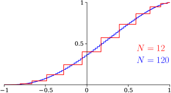
Figure 18.40.1: Histogram approximations to the Repulsive Coulomb–Pollaczek, RCP, weight function integrated over $[-1,x)$, see Figure 18.39.2 for an exact result, for $Z=+1$, shown for $N=12$ and $N=120$. Magnify

… ►This is a challenging case as the desired $w^{\mathrm{RCP}}(x)$ on $[-1,1]$ has an essential singularity at $x=-1$. … ►Further, exponential convergence in $N$, via the Derivative Rule, rather than the power-law convergence of the histogram methods, is found for the inversion of Gegenbauer, Attractive, as well as Repulsive, Coulomb–Pollaczek, and Hermite weights and zeros to approximate $w(x)$ for these OP systems on $x\in [-1,1]$ and $(-\mathrm{\infty },\mathrm{\infty })$ respectively, Reinhardt (2018), and Reinhardt (2021b), Reinhardt (2021a). …

16: 4.23 Inverse Trigonometric Functions

… ►

4.23.20 $$\arcsin x=\frac{1}{2}\pi \pm \mathrm{i}\ln \left({(x^2-1)}^{1/2}+x\right),$$ $x\in [1,\mathrm{\infty })$,

ⓘ

Symbols:

$\pi$: the ratio of the circumference of a circle to its diameter, $[a,b)$: half-closed interval, $\in$: element of, $\mathrm{i}$: imaginary unit, $\arcsin z$: arcsine function, $\ln z$: principal branch of logarithm function and $x$: real variable

Permalink:

http://dlmf.nist.gov/4.23.E20

Encodings:

pMML, png, TeX

See also:

Annotations for §4.23(iv), §4.23(iv), §4.23 and Ch.4

►

4.23.21 $$\arcsin x=-\frac{1}{2}\pi \pm \mathrm{i}\ln \left({(x^2-1)}^{1/2}-x\right),$$ $x\in (-\mathrm{\infty },-1]$,

ⓘ

Symbols:

$\pi$: the ratio of the circumference of a circle to its diameter, $\in$: element of, $\mathrm{i}$: imaginary unit, $\arcsin z$: arcsine function, $\ln z$: principal branch of logarithm function, $(a,b]$: half-closed interval and $x$: real variable

Permalink:

http://dlmf.nist.gov/4.23.E21

Encodings:

pMML, png, TeX

See also:

Annotations for §4.23(iv), §4.23(iv), §4.23 and Ch.4

… ►

4.23.24 $$\arccos x=\mp \mathrm{i}\ln \left({(x^2-1)}^{1/2}+x\right),$$ $x\in [1,\mathrm{\infty })$,

ⓘ

Symbols:

$[a,b)$: half-closed interval, $\in$: element of, $\mathrm{i}$: imaginary unit, $\arccos z$: arccosine function, $\ln z$: principal branch of logarithm function and $x$: real variable

Permalink:

http://dlmf.nist.gov/4.23.E24

Encodings:

pMML, png, TeX

See also:

Annotations for §4.23(iv), §4.23(iv), §4.23 and Ch.4

►

4.23.25 $$\arccos x=\pi \mp \mathrm{i}\ln \left({(x^2-1)}^{1/2}-x\right),$$ $x\in (-\mathrm{\infty },-1]$,

ⓘ

Symbols:

$\pi$: the ratio of the circumference of a circle to its diameter, $\in$: element of, $\mathrm{i}$: imaginary unit, $\arccos z$: arccosine function, $\ln z$: principal branch of logarithm function, $(a,b]$: half-closed interval and $x$: real variable

Permalink:

http://dlmf.nist.gov/4.23.E25

Encodings:

pMML, png, TeX

See also:

Annotations for §4.23(iv), §4.23(iv), §4.23 and Ch.4

… ►

4.23.26 $$\arctan z=\frac{\mathrm{i}}{2}\ln \left(\frac{\mathrm{i}+z}{\mathrm{i}-z}\right),$$ $z/\mathrm{i}\in ℂ\setminus (-\mathrm{\infty },-1]\cup [1,\mathrm{\infty })$;

ⓘ

Symbols:

$[a,b)$: half-closed interval, $ℂ$: complex plane, $\in$: element of, $\mathrm{i}$: imaginary unit, $\arctan z$: arctangent function, $\ln z$: principal branch of logarithm function, $(a,b]$: half-closed interval, $\setminus$: set subtraction, $\cup$: union and $z$: complex variable

Referenced by:

§4.23(iv)

Permalink:

http://dlmf.nist.gov/4.23.E26

Encodings:

pMML, png, TeX

See also:

Annotations for §4.23(iv), §4.23(iv), §4.23 and Ch.4

…

17: 1.4 Calculus of One Variable

… ►Suppose $f(x)$ is defined on $[a,b]$. …Continuity, or piecewise continuity, of $f(x)$ on $[a,b]$ is sufficient for the limit to exist. … ►For $f(x)$ continuous and $\varphi (x)\ge 0$ and integrable on $[a,b]$, there exists $c\in [a,b]$, such that … ►If $f(x)$ is continuous or piecewise continuous on $[a,b]$, then … ►A similar definition applies to closed intervals $[a,b]$. …

18: 7.24 Approximations

… ►

Schonfelder (1978) gives coefficients of Chebyshev expansions for $x^{-1}\mathrm{erf}x$ on $0\le x\le 2$, for $x{\mathrm{e}}^{x^2}\mathrm{erfc}x$ on $[2,\mathrm{\infty })$, and for ${\mathrm{e}}^{x^2}\mathrm{erfc}x$ on $[0,\mathrm{\infty })$ (30D).

…

19: 8.1 Special Notation

… ►Alternative notations include: Prym’s functions $P_z(a)=\gamma (a,z)$, $Q_z(a)=\mathrm{\Gamma }(a,z)$, Nielsen (1906a, pp. 25–26), Batchelder (1967, p. 63); $(a,z)!=\gamma (a+1,z)$, $[a,z]!=\mathrm{\Gamma }(a+1,z)$, Dingle (1973); $B(a,b,x)={\mathrm{B}}_x(a,b)$, $I(a,b,x)=I_x(a,b)$, Magnus et al. (1966); $\mathrm{Si}(a,x)\to \mathrm{Si}(1-a,x)$, $\mathrm{Ci}(a,x)\to \mathrm{Ci}(1-a,x)$, Luke (1975).

20: 22.1 Special Notation

… ► ►►►

$x,y$	real variables.
…
$k^{\prime }$	complementary modulus, $k^2+k_{}^{\prime }{}_{}{}^2=1$. If $k\in [0,1]$, then $k^{\prime }\in [0,1]$.
…

…