DLMF: Untitled Document

(a)

$A\sin a$ , $A\sin\left(a+\frac{2}{3}\pi\right)$ , and $A\sin\left(a+\frac{4}{3}\pi\right)$ , with $\sin\left(3a\right)=C$ , when $p<0$ and $C\leq 1$ .
(b)

$A\cosh a$ , $A\cosh\left(a+\frac{2}{3}\pi i\right)$ , and $A\cosh\left(a+\frac{4}{3}\pi i\right)$ , with $\cosh\left(3a\right)=C$ , when $p<0$ and $C>1$ .
(c)

$B\sinh a$ , $B\sinh\left(a+\frac{2}{3}\pi i\right)$ , and $B\sinh\left(a+\frac{4}{3}\pi i\right)$ , with $\sinh\left(3a\right)=D$ , when $p>0$ .

Reported 2014-10-31 by Masataka Urago

See also:

Annotations for §4.43 and Ch.4

… ►

(a)

$A\sin a$ , $A\sin\left(a+\frac{2}{3}\pi\right)$ , and $A\sin\left(a+\frac{4}{3}\pi\right)$ , with $\sin\left(3a\right)=4q/A^{3}$ , when $4p^{3}+27q^{2}\leq 0$ .

►

(b)

$A\cosh a$ , $A\cosh\left(a+\frac{2}{3}\pi i\right)$ , and $A\cosh\left(a+\frac{4}{3}\pi i\right)$ , with $\cosh\left(3a\right)=-4q/A^{3}$ , when $p<0$ , $q<0$ , and $4p^{3}+27q^{2}>0$ .

►

(c)

$B\sinh a$ , $B\sinh\left(a+\frac{2}{3}\pi i\right)$ , and $B\sinh\left(a+\frac{4}{3}\pi i\right)$ , with $\sinh\left(3a\right)=-4q/B^{3}$ , when $p>0$ .

►Note that in Case (a) all the roots are real, whereas in Cases (b) and (c) there is one real root and a conjugate pair of complex roots. …

… ►

6.9.1

E_{1}\left(z\right)=\cfrac{e^{-z}}{z+\cfrac{1}{1+\cfrac{1}{z+\cfrac{2}{1+% \cfrac{2}{z+\cfrac{3}{1+\cfrac{3}{z+}}}}}}}\cdots,

|\operatorname{ph}z|<\pi

.

ⓘ

Symbols:: $\pi$ : the ratio of the circumference of a circle to its diameter, $\mathrm{e}$ : base of natural logarithm, $E_{1}\left(\NVar{z}\right)$ : exponential integral, $\operatorname{ph}$ : phase and $z$ : complex variable
A&S Ref:: 5.1.22 (special case of)
Referenced by:: §6.18(i)
Permalink:: http://dlmf.nist.gov/6.9.E1
Encodings:: pMML, png, TeX
See also:: Annotations for §6.9 and Ch.6

…

… ►However, in the case of

\operatorname{Ai}\left(z\right)

and

\operatorname{Bi}\left(z\right)

this accuracy can be increased considerably by use of the exponentially-improved forms of expansion supplied in §9.7(v). … ►In the case of

\operatorname{Ai}\left(z\right)

, for example, this means that in the sectors

\tfrac{1}{3}\pi<|\operatorname{ph}z|<\pi

we may integrate along outward rays from the origin with initial values obtained from §9.2(ii). …On the remaining rays, given by

\operatorname{ph}z=\pm\tfrac{1}{3}\pi

and

\pi

, integration can proceed in either direction. … ►In the case of the Scorer functions, integration of the differential equation (9.12.1) is more difficult than (9.2.1), because in some regions stable directions of integration do not exist. …In these cases boundary-value methods need to be used instead; see §3.7(iii). …

… ►

23.7.1

\wp\left(\tfrac{1}{2}\omega_{1}\right)=e_{1}+\sqrt{(e_{1}-e_{3})(e_{1}-e_{2})}% =e_{1}+\omega_{1}^{-2}(K\left(k\right))^{2}k^{\prime},

ⓘ

Symbols:: $\wp\left(\NVar{z}\right)$ (= $\wp\left(z|\mathbb{L}\right)$ = $\wp\left(z;g_{2},g_{3}\right)$ ): Weierstrass $\wp$ -function, $e_{\NVar{j}}$ : Weierstrass lattice roots, $K\left(\NVar{k}\right)$ : Legendre’s complete elliptic integral of the first kind, $\mathbb{L}$ : lattice, $\omega_{1}$ , $\omega_{3}$ , $\omega_{2}=-\omega_{1}-\omega_{3}$ : lattice generators, $k$ : modulus and $k^{\prime}$ : complementary modulus
A&S Ref:: 18.3.18
Permalink:: http://dlmf.nist.gov/23.7.E1
Encodings:: pMML, png, TeX
See also:: Annotations for §23.7 and Ch.23

►

23.7.2

\wp\left(\tfrac{1}{2}\omega_{2}\right)=e_{2}-i\sqrt{(e_{1}-e_{2})(e_{2}-e_{3})% }=e_{2}-i\omega_{1}^{-2}(K\left(k\right))^{2}kk^{\prime},

ⓘ

Symbols:: $\wp\left(\NVar{z}\right)$ (= $\wp\left(z|\mathbb{L}\right)$ = $\wp\left(z;g_{2},g_{3}\right)$ ): Weierstrass $\wp$ -function, $e_{\NVar{j}}$ : Weierstrass lattice roots, $K\left(\NVar{k}\right)$ : Legendre’s complete elliptic integral of the first kind, $\mathrm{i}$ : imaginary unit, $\mathbb{L}$ : lattice, $\omega_{1}$ , $\omega_{3}$ , $\omega_{2}=-\omega_{1}-\omega_{3}$ : lattice generators, $k$ : modulus and $k^{\prime}$ : complementary modulus
A&S Ref:: 18.3.18
Permalink:: http://dlmf.nist.gov/23.7.E2
Encodings:: pMML, png, TeX
See also:: Annotations for §23.7 and Ch.23

►

23.7.3

\wp\left(\tfrac{1}{2}\omega_{3}\right)=e_{3}-\sqrt{(e_{1}-e_{3})(e_{2}-e_{3})}% =e_{3}-\omega_{1}^{-2}(K\left(k\right))^{2}k,

ⓘ

Symbols:: $\wp\left(\NVar{z}\right)$ (= $\wp\left(z|\mathbb{L}\right)$ = $\wp\left(z;g_{2},g_{3}\right)$ ): Weierstrass $\wp$ -function, $e_{\NVar{j}}$ : Weierstrass lattice roots, $K\left(\NVar{k}\right)$ : Legendre’s complete elliptic integral of the first kind, $\mathbb{L}$ : lattice, $\omega_{1}$ , $\omega_{3}$ , $\omega_{2}=-\omega_{1}-\omega_{3}$ : lattice generators and $k$ : modulus
A&S Ref:: 18.3.18
Permalink:: http://dlmf.nist.gov/23.7.E3
Encodings:: pMML, png, TeX
See also:: Annotations for §23.7 and Ch.23

►where

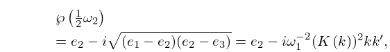
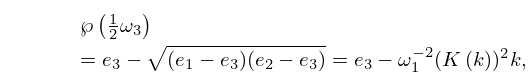
k,k^{\prime}

and the square roots are real and positive when the lattice is rectangular; otherwise they are determined by continuity from the rectangular case.

… ►

7.8.4

\mathsf{M}\left(x\right)<\frac{2}{3x+\sqrt{x^{2}+4}},

x>-\tfrac{1}{2}\sqrt{2}

,

ⓘ

Symbols:: $\mathsf{M}\left(\NVar{x}\right)$ : Mills’ ratio and $x$ : real variable
Referenced by:: §7.8
Permalink:: http://dlmf.nist.gov/7.8.E4
Encodings:: pMML, png, TeX
See also:: Annotations for §7.8 and Ch.7

►

7.8.5

\frac{x^{2}}{2x^{2}+1}\leq\frac{x^{2}(2x^{2}+5)}{4x^{4}+12x^{2}+3}\leq x% \mathsf{M}\left(x\right)<\frac{2x^{4}+9x^{2}+4}{4x^{4}+20x^{2}+15}<\frac{x^{2}% +1}{2x^{2}+3},

x\geq 0

.

ⓘ

Symbols:: $\mathsf{M}\left(\NVar{x}\right)$ : Mills’ ratio and $x$ : real variable
Referenced by:: §7.8
Permalink:: http://dlmf.nist.gov/7.8.E5
Encodings:: pMML, png, TeX
See also:: Annotations for §7.8 and Ch.7

… ►

7.8.6

\int_{0}^{x}e^{at^{2}}\,\mathrm{d}t<\frac{1}{3ax}\left(2e^{ax^{2}}+ax^{2}-2% \right),

a,x>0

.

ⓘ

Symbols:: $\,\mathrm{d}\NVar{x}$ : differential of $x$ , $\mathrm{e}$ : base of natural logarithm, $\int$ : integral and $x$ : real variable
Referenced by:: §7.8
Permalink:: http://dlmf.nist.gov/7.8.E6
Encodings:: pMML, png, TeX
See also:: Annotations for §7.8 and Ch.7

… ►

7.8.8

\operatorname{erf}x<\sqrt{1-{\mathrm{e}}^{-4x^{2}/\pi}},

x>0

.

ⓘ

Symbols:: $\pi$ : the ratio of the circumference of a circle to its diameter, $\operatorname{erf}\NVar{z}$ : error function, $\mathrm{e}$ : base of natural logarithm and $x$ : real variable
Source:: Pólya (1949, (1.5))
Referenced by:: §7.8, Erratum (V1.0.17) for Equation (7.8.8)
Permalink:: http://dlmf.nist.gov/7.8.E8
Encodings:: pMML, png, TeX
Addition (effective with 1.0.17):: This inequality was added. It is Pólya (1949, (1.5)). Note that it is a special case of (8.10.11).
Suggested by Roberto Iacono
See also:: Annotations for §7.8 and Ch.7

… ►This has regular singularities at

z=0

and

1

, and an irregular singularity of rank 1 at

z=\infty

. ►Mathieu functions (Chapter 28), spheroidal wave functions (Chapter 30), and Coulomb spheroidal functions (§30.12) are special cases of solutions of the confluent Heun equation. … ►This has one singularity, an irregular singularity of rank

3

at

z=\infty

. …

… ►

…

Figure 26.9.1: Ferrers graph of the partition

7+4+3+3+2+1

.

… ►

Figure 26.9.2: The partition

5+5+3+2

represented as a lattice path.

… ►

p_{3}\left(n\right)=1+\left\lfloor\frac{n^{2}+6n}{12}\right\rfloor.

… ►In the present chapter

m\geq n\geq 0

in all cases. … ►equivalently, partitions into at most

k

parts either have exactly

k

parts, in which case we can subtract one from each part, or they have strictly fewer than

k

parts. …

… ►If

-\tfrac{3}{2}<a<-\tfrac{1}{2}

, then

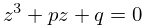
U\left(a,x\right)

has no positive real zeros. If

-2n-\tfrac{3}{2}<a<-2n+\tfrac{1}{2}

,

n=1,2,\dots

, then

U\left(a,x\right)

has

n

positive real zeros. Lastly, when

a=-n-\tfrac{1}{2}

,

n=1,2,\dots

(Hermite polynomial case)

U\left(a,x\right)

has

n

zeros and they lie in the interval

[-2\sqrt{-a},2\sqrt{-a}\,]

. For further information on these cases see Dean (1966). … ►Numerical calculations in this case show that

z_{\frac{1}{2},s}

corresponds to the

s

th zero on the string; compare §7.13(ii). …

… ►The computation is slowest for complete cases. … ►Complete cases of Legendre’s integrals and symmetric integrals can be computed with quadratic convergence by the AGM method (including Bartky transformations), using the equations in §19.8(i) and §19.22(ii), respectively. … ►The step from

n

to

n+1

is an ascending Landen transformation if

\theta=1

(leading ultimately to a hyperbolic case of

R_{C}

) or a descending Gauss transformation if

\theta=-1

(leading to a circular case of

R_{C}

). … ►Also, see Todd (1975) for a special case of

K\left(k\right)

. For computation of Legendre’s integral of the third kind, see Abramowitz and Stegun (1964, §§17.7 and 17.8, Examples 15, 17, 19, and 20). …

… ►

D. Naylor (1989) On an integral transform involving a class of Mathieu functions. SIAM J. Math. Anal. 20 (6), pp. 1500–1513.

ⓘ

External Links:: ISSN 0036-1410, Document, MathReview (K. C. Gupta), ZentralBlatt
Referenced by:: §28.26(ii).
Encodings:: BibTeX

… ►

D. Naylor (1996) On an asymptotic expansion of the Kontorovich-Lebedev transform. Methods Appl. Anal. 3 (1), pp. 98–108.

ⓘ

External Links:: ISSN 1073-2772, FullText, MathReview (C. M. Joshi), ZentralBlatt
Referenced by:: §10.43(v).
Encodings:: BibTeX

… ►

W. J. Nellis and B. C. Carlson (1966) Reduction and evaluation of elliptic integrals. Math. Comp. 20 (94), pp. 223–231.

ⓘ

External Links:: FullText, MathReview (I. A. Stegun), ZentralBlatt
Referenced by:: §19.37(iv).
Encodings:: BibTeX

… ►

P. Nevai (1986) Géza Freud, orthogonal polynomials and Christoffel functions. A case study. J. Approx. Theory 48 (1), pp. 3–167.

ⓘ

External Links:: ISSN 0021-9045, Document, MathReview (T. S. Chihara), ZentralBlatt
Referenced by:: §18.32.
Encodings:: BibTeX

… ►

E. W. Ng and M. Geller (1969) A table of integrals of the error functions. J. Res. Nat. Bur. Standards Sect B. 73B, pp. 1–20.

ⓘ

Notes:: See for additions and corrections same journal, Sect. B 75, 149–163 (1975)
External Links:: MathReview, ZentralBlatt
Referenced by:: §7.14(iii), §7.21, §7.7(iii).
Encodings:: BibTeX

…

case%20%CE%BB%3D0

11—20 of 664 matching pages

11: 4.43 Cubic Equations

12: 6.9 Continued Fraction

13: 9.17 Methods of Computation

14: 23.7 Quarter Periods

15: 7.8 Inequalities

16: 31.12 Confluent Forms of Heun’s Equation

17: 26.9 Integer Partitions: Restricted Number and Part Size

18: 12.11 Zeros

19: 19.36 Methods of Computation

20: Bibliography N