asymptotic approximations for coefficients

SearchAdvancedHelp

(0.005 seconds)

11—20 of 57 matching pages

11: 2.3 Integrals of a Real Variable

… ►For the Fourier integral … ►

§2.3(ii) Watson’s Lemma

… ►

§2.3(iv) Method of Stationary Phase

… ►

§2.3(v) Coalescing Peak and Endpoint: Bleistein’s Method

… ►

§2.3(vi) Asymptotics of Mellin Transforms

…

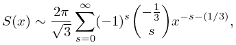
12: 26.7 Set Partitions: Bell Numbers

… ►

26.7.6 $$B\left(n+1\right)=\sum _{k=0}^n\left(\genfrac{}{}{0.0pt}{}{n}{k}\right)B\left(k\right).$$

ⓘ

Symbols:

$B\left(n\right)$: Bell number, $\left(\genfrac{}{}{0.0pt}{}{m}{n}\right)$: binomial coefficient, $k$: nonnegative integer and $n$: nonnegative integer

Referenced by:

Erratum (V1.0.1) for Equation (26.7.6)

Permalink:

http://dlmf.nist.gov/26.7.E6

Encodings:

pMML, png, TeX

Errata (effective with 1.0.1):

Originally appeared with $B\left(n\right)$ in the summation, instead of $B\left(k\right)$:

$$B\left(n+1\right)=\sum _{k=0}^n\left(\genfrac{}{}{0.0pt}{}{n}{k}\right)B\left(n\right)$$

Reported 2010-11-07 by Layne Watson

See also:

Annotations for §26.7(iii), §26.7 and Ch.26

►

§26.7(iv) Asymptotic Approximation

… ►For higher approximations to $B\left(n\right)$ as $n\to \mathrm{\infty }$ see de Bruijn (1961, pp. 104–108).

13: 2.4 Contour Integrals

… ►

§2.4(i) Watson’s Lemma

… ►For examples see Olver (1997b, pp. 315–320). ►

§2.4(iii) Laplace’s Method

… ►

§2.4(v) Coalescing Saddle Points: Chester, Friedman, and Ursell’s Method

… ►

§2.4(vi) Other Coalescing Critical Points

…

14: 8.12 Uniform Asymptotic Expansions for Large Parameter

§8.12 Uniform Asymptotic Expansions for Large Parameter

… ►With $\mu =\lambda -1$, the coefficients $c_k(\eta )$ are given by …where $g_k$, $k=0,1,2,\mathrm{\dots }$, are the coefficients that appear in the asymptotic expansion (5.11.3) of $\mathrm{\Gamma }\left(z\right)$. … ►For other uniform asymptotic approximations of the incomplete gamma functions in terms of the function $\mathrm{erfc}$ see Paris (2002b) and Dunster (1996a). ►

Inverse Function

…

15: 2.6 Distributional Methods

… ►

2.6.6 $$S(x)\sim \frac{2\pi }{\sqrt{3}}\sum _{s=0}^{\mathrm{\infty }}{(-1)}^s\left(\genfrac{}{}{0.0pt}{}{-\frac{1}{3}}{s}\right)x^{-s-(1/3)},$$ $x\to \mathrm{\infty }$.

ⓘ

Symbols:

$\sim$: Poincaré asymptotic expansion, $\left(\genfrac{}{}{0.0pt}{}{m}{n}\right)$: binomial coefficient, $\pi$: the ratio of the circumference of a circle to its diameter and $S(x)$: integral

Referenced by:

§2.6(i)

Permalink:

http://dlmf.nist.gov/2.6.E6

Encodings:

pMML, png, TeX

See also:

Annotations for §2.6(i), §2.6 and Ch.2

…

16: 28.25 Asymptotic Expansions for Large $\mathrm{\Re }z$

§28.25 Asymptotic Expansions for Large $\mathrm{\Re }z$

… ►

28.25.1 $${\mathrm{M}}_{\nu }^{(3,4)}(z,h)\sim \frac{{\mathrm{e}}^{\pm \mathrm{i}\left(2h\cosh z-\left(\frac{1}{2}\nu +\frac{1}{4}\right)\pi \right)}}{{\left(\pi h(\cosh z+1)\right)}^{\frac{1}{2}}}\sum _{m=0}^{\mathrm{\infty }}\frac{D_m^{\pm }}{{\left(\mp 4\mathrm{i}h(\cosh z+1)\right)}^m},$$

ⓘ

Symbols:

$\sim$: Poincaré asymptotic expansion, $\pi$: the ratio of the circumference of a circle to its diameter, $\mathrm{e}$: base of natural logarithm, $\cosh z$: hyperbolic cosine function, $\mathrm{i}$: imaginary unit, ${\mathrm{M}}_{\nu }^{(j)}(z,h)$: modified Mathieu function, $m$: integer, $h$: parameter, $z$: complex variable, $\nu$: complex parameter and $D_m^{\pm }$: coefficients

A&S Ref:

20.9.1 (for 3 and for integer $\nu$) 20.9.3 (for 4 and for integer $\nu$)

Referenced by:

§28.25

Permalink:

http://dlmf.nist.gov/28.25.E1

Encodings:

pMML, png, TeX

See also:

Annotations for §28.25 and Ch.28

►where the coefficients are given by … ►

28.25.3 $$(m+1)D_{m+1}^{\pm }+\left({(m+\frac{1}{2})}^2\pm (m+\frac{1}{4})8\mathrm{i}h+2h^2-a\right)D_m^{\pm }\pm (m-\frac{1}{2})\left(8\mathrm{i}hm\right)D_{m-1}^{\pm }=0,$$ $m\ge 0$.

ⓘ

Symbols:

$\mathrm{i}$: imaginary unit, $m$: integer, $h$: parameter, $a$: parameter and $D_m^{\pm }$: coefficients

A&S Ref:

20.9.2 (for $+$) 20.9.4 (for $-$)

Permalink:

http://dlmf.nist.gov/28.25.E3

Encodings:

pMML, png, TeX

See also:

Annotations for §28.25 and Ch.28

…

17: 28.34 Methods of Computation

… ►

Use of asymptotic expansions and approximations for large $q$ (§§28.8(i), 28.16). See also Zhang and Jin (1996, pp. 482–485).

… ►

Solution of the continued-fraction equations (28.6.16)–(28.6.19) and (28.15.2) by successive approximation. See Blanch (1966), Shirts (1993a), and Meixner and Schäfke (1954, §2.87).

►

Asymptotic approximations by zeros of orthogonal polynomials of increasing degree. See Volkmer (2008). This method also applies to eigenvalues of the Whittaker–Hill equation (§28.31(i)) and eigenvalues of Lamé functions (§29.3(i)).

… ►

Use of asymptotic expansions and approximations for large $q$ (§§28.8(ii)–28.8(iv)).

… ►

Use of asymptotic expansions for large $z$ or large $q$. See §§28.25 and 28.26.

18: 30.9 Asymptotic Approximations and Expansions

§30.9 Asymptotic Approximations and Expansions

… ►Further coefficients can be found with the Maple program SWF7; see §30.18(i). … ►Further coefficients can be found with the Maple program SWF8; see §30.18(i). … ►

§30.9(iii) Other Approximations and Expansions

… ►

19: 10.41 Asymptotic Expansions for Large Order

§10.41 Asymptotic Expansions for Large Order

►

§10.41(i) Asymptotic Forms

… ►

§10.41(iv) Double Asymptotic Properties

… ►

§10.41(v) Double Asymptotic Properties (Continued)

… ►

20: 10.21 Zeros

… ►The approximations that follow in §10.21(viii) do not suffer from this drawback. ►

§10.21(viii) Uniform Asymptotic Approximations for Large Order

… ►The latter reference includes numerical tables of the first few coefficients in the uniform asymptotic expansions. … ►Higher coefficients in the asymptotic expansions in this subsection can be obtained by expressing the cross-products in terms of the modulus and phase functions (§10.18), and then reverting the asymptotic expansion for the difference of the phase functions. … ►This information includes asymptotic approximations analogous to those given in §§10.21(vi), 10.21(vii), and 10.21(x). …