…
►where the are monic polynomials (coefficient of highest power of is ) satisfying
…with , .
…
►Next, let be the polynomials defined by for , and
…where is the Wronskian determinant
…
►where and are polynomials of degree , with no common zeros.
…
…
►The Stokes set takes different forms for , , and .
►For , the set consists of the two curves
…
►For , the Stokes set is expressed in terms of scaled coordinates
…
►For , there are two solutions , provided that .
…
►For the Stokes set has two sheets.
…
Zhang and Jin (1996, pp. 455–473) includes
, ,
, , and
derivatives,
, , , 8S;
, , and derivatives,
, and , , , 8S.
Also, first zeros of
, , and of derivatives, , 6D;
first three zeros of
and of derivative, , 6D;
first three zeros of
and of derivative, , 6D;
real and imaginary parts of , ,
, , , 8S.
…
►Elliptic umbilic bifurcation set (codimension three): for fixed , the section of the bifurcation set is a three-cusped astroid
…
►The sign labels the cusped sheet; the sign labels the sheet that is smooth for (see Figure 36.4.4).
…
…
►Their product has 20 digits, twice the number of digits in the data.
…These numbers, in turn, are combined by the Chinese remainder theorem to obtain the final result , which is correct to 20 digits.
…
 ►
►
