along%20real%20line

SearchAdvancedHelp

(0.003 seconds)

11—20 of 684 matching pages

11: Bibliography P

… ►

Interlacing of positive real zeros of Bessel functions. J. Math. Anal. Appl. 375 (1), pp. 320–322.

ⓘ

External Links:

ISSN 0022-247X, Document, FullText, MathReview (Javier Segura), ZentralBlatt

Referenced by:

§10.21(i), §10.21(i).

Encodings:

BibTeX

… ►

Influence of equilibrium shear flow along the magnetic field on the resistive tearing instability. Phys. Fluids 26 (10), pp. 2966–2975.

ⓘ

External Links:

ISSN 0031-9171, Document, MathReview, ZentralBlatt

Referenced by:

§11.12, §11.7(ii).

Encodings:

BibTeX

… ►

On the use of Hadamard expansions in hyperasymptotic evaluation. I. Real variables. Proc. Roy. Soc. London Ser. A 457 (2016), pp. 2835–2853.

ⓘ

External Links:

ISSN 1364-5021, Document, MathReview (Andrea Laforgia), ZentralBlatt

Referenced by:

§10.40(iv), §2.11(v).

Encodings:

BibTeX

… ►

Automatic computation of Bessel function integrals. Comput. Phys. Comm. 25 (3), pp. 289–295.

ⓘ

Notes:

Double-precision Fortran, maximum accuracy 20S.

External Links:

ISSN 0010-4655, Document, Code

Referenced by:

6th item.

Encodings:

BibTeX

… ►

Fast analytic formulas for the modified Bessel functions of imaginary order for spectral line broadening calculations. J. Quantit. Spec. and Rad. Trans. 62 (4), pp. 389–395.

ⓘ

External Links:

Document

Referenced by:

§10.76(ii).

Encodings:

BibTeX

…

12: 4.15 Graphics

… ►

§4.15(i) Real Arguments

… ►Figure 4.15.7 illustrates the conformal mapping of the strip onto the whole $w$-plane cut along the real axis from $-\mathrm{\infty }$ to $-1$ and $1$ to $\mathrm{\infty }$, where $w=\sin z$ and $z=\arcsin w$ (principal value). …Lines parallel to the real axis in the $z$-plane map onto ellipses in the $w$-plane with foci at $w=\pm 1$, and lines parallel to the imaginary axis in the $z$-plane map onto rectangular hyperbolas confocal with the ellipses. In the labeling of corresponding points $r$ is a real parameter that can lie anywhere in the interval $(0,\mathrm{\infty })$. … ►

►

►

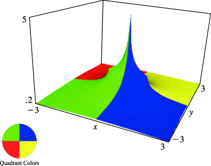
Figure 4.15.13: $\mathrm{arccsc}\left(x+\mathrm{i}y\right)$ (principal value). There is a branch cut along the real axis from $-1$ to $1$. Magnify 3D Help

…

13: 13.16 Integral Representations

… ►

§13.16(i) Integrals Along the Real Line

… ►

13.16.3 $$\frac{1}{\mathrm{\Gamma }\left(1+2\mu \right)}{M}_{\kappa ,\mu }\left(z\right)=\frac{\sqrt{z}{\mathrm{e}}^{\frac{1}{2}z}}{\mathrm{\Gamma }\left(\frac{1}{2}+\mu +\kappa \right)}{\int }_0^{\mathrm{\infty }}{\mathrm{e}}^{-t}{t}^{\kappa -\frac{1}{2}}{J}_{2\mu }\left(2\sqrt{zt}\right)dt,$$ $\mathrm{\Re }\left(\kappa +\mu \right)+\frac{1}{2}>0$,

ⓘ

Symbols:

$J_{\nu }\left(z\right)$: Bessel function of the first kind, $\mathrm{\Gamma }\left(z\right)$: gamma function, $M_{\kappa ,\mu }\left(z\right)$: Whittaker confluent hypergeometric function, $dx$: differential of $x$ , $\mathrm{e}$: base of natural logarithm, $\int$: integral, $\mathrm{\Re }$: real part and $z$: complex variable

Permalink:

http://dlmf.nist.gov/13.16.E3

Encodings:

pMML, png, TeX

See also:

Annotations for §13.16(i), §13.16 and Ch.13

►

13.16.4 $$\frac{1}{\mathrm{\Gamma }\left(1+2\mu \right)}{M}_{\kappa ,\mu }\left(z\right)=\frac{\sqrt{z}{\mathrm{e}}^{-\frac{1}{2}z}}{\mathrm{\Gamma }\left(\frac{1}{2}+\mu -\kappa \right)}{\int }_0^{\mathrm{\infty }}{\mathrm{e}}^{-t}{t}^{-\kappa -\frac{1}{2}}{I}_{2\mu }\left(2\sqrt{zt}\right)dt,$$ .

ⓘ

Symbols:

$\mathrm{\Gamma }\left(z\right)$: gamma function, $M_{\kappa ,\mu }\left(z\right)$: Whittaker confluent hypergeometric function, $dx$: differential of $x$ , $\mathrm{e}$: base of natural logarithm, $\int$: integral, $I_{\nu }\left(z\right)$: modified Bessel function of the first kind, $\mathrm{\Re }$: real part and $z$: complex variable

Referenced by:

Erratum (V1.0.5) for Equation (13.16.4)

Permalink:

http://dlmf.nist.gov/13.16.E4

Encodings:

pMML, png, TeX

Errata (effective with 1.0.5):

Originally the condition for the validity of this equation was stated incorrectly as $\mathrm{\Re }(\kappa -\mu )-\frac{1}{2}>0$. The correct condition is .

See also:

Annotations for §13.16(i), §13.16 and Ch.13

… ►where $c$ is arbitrary, $\mathrm{\Re }c>0$. …

14: 9.17 Methods of Computation

… ►As described in §3.7(ii), to ensure stability the integration path must be chosen in such a way that as we proceed along it the wanted solution grows at least as fast as all other solutions of the differential equation. In the case of $\mathrm{Ai}\left(z\right)$, for example, this means that in the sectors we may integrate along outward rays from the origin with initial values obtained from §9.2(ii). … ►An example is provided by $\mathrm{Gi}\left(x\right)$ on the positive real axis. … ►Among the integral representations of the Airy functions the Stieltjes transform (9.10.18) furnishes a way of computing $\mathrm{Ai}\left(z\right)$ in the complex plane, once values of this function can be generated on the positive real axis. …

15: 8 Incomplete Gamma and Related
Functions

…

16: 28 Mathieu Functions and Hill’s Equation

…

17: 11.5 Integral Representations

… ►

§11.5(i) Integrals Along the Real Line

… ►

11.5.2 $${𝐊}_{\nu }\left(z\right)=\frac{2{(\frac{1}{2}z)}^{\nu }}{\sqrt{\pi }\mathrm{\Gamma }\left(\nu +\frac{1}{2}\right)}{\int }_0^{\mathrm{\infty }}{\mathrm{e}}^{-zt}{(1+t^2)}^{\nu -\frac{1}{2}}dt,$$ $\mathrm{\Re }z>0$,

ⓘ

Symbols:

$\mathrm{\Gamma }\left(z\right)$: gamma function, ${𝐊}_{\nu }\left(z\right)$: Struve function, $\pi$: the ratio of the circumference of a circle to its diameter, $dx$: differential of $x$ , $\mathrm{e}$: base of natural logarithm, $\int$: integral, $\mathrm{\Re }$: real part, $z$: complex variable and $\nu$: real or complex order

A&S Ref:

12.1.8

Referenced by:

§11.13(iii), §11.5(i), §11.5(ii), §11.6(i)

Permalink:

http://dlmf.nist.gov/11.5.E2

Encodings:

pMML, png, TeX

See also:

Annotations for §11.5(i), §11.5 and Ch.11

… ►

11.5.4 $${𝐌}_{\nu }\left(z\right)=-\frac{2{(\frac{1}{2}z)}^{\nu }}{\sqrt{\pi }\mathrm{\Gamma }\left(\nu +\frac{1}{2}\right)}{\int }_0^1{\mathrm{e}}^{-zt}{(1-t^2)}^{\nu -\frac{1}{2}}dt,$$ $\mathrm{\Re }\nu >-\frac{1}{2}$,

ⓘ

Symbols:

$\mathrm{\Gamma }\left(z\right)$: gamma function, ${𝐌}_{\nu }\left(z\right)$: modified Struve function, $\pi$: the ratio of the circumference of a circle to its diameter, $dx$: differential of $x$ , $\mathrm{e}$: base of natural logarithm, $\int$: integral, $\mathrm{\Re }$: real part, $z$: complex variable and $\nu$: real or complex order

Referenced by:

§11.5(i), §11.5(ii), §11.6(i), §11.6(iii)

Permalink:

http://dlmf.nist.gov/11.5.E4

Encodings:

pMML, png, TeX

See also:

Annotations for §11.5(i), §11.5 and Ch.11

… ►

11.5.7 $$I_{-\nu }\left(x\right)-{𝐋}_{\nu }\left(x\right)=\frac{2{(\frac{1}{2}x)}^{\nu }}{\sqrt{\pi }\mathrm{\Gamma }\left(\nu +\frac{1}{2}\right)}{\int }_0^{\mathrm{\infty }}{(1+t^2)}^{\nu -\frac{1}{2}}\sin \left(xt\right)dt,$$ $x>0$, .

ⓘ

Symbols:

$\mathrm{\Gamma }\left(z\right)$: gamma function, $\pi$: the ratio of the circumference of a circle to its diameter, $dx$: differential of $x$ , $\int$: integral, $I_{\nu }\left(z\right)$: modified Bessel function of the first kind, ${𝐋}_{\nu }\left(z\right)$: modified Struve function, $\mathrm{\Re }$: real part, $\sin z$: sine function, $x$: real variable and $\nu$: real or complex order

Referenced by:

§11.5(i), §11.5(ii)

Permalink:

http://dlmf.nist.gov/11.5.E7

Encodings:

pMML, png, TeX

See also:

Annotations for §11.5(i), §11.5 and Ch.11

… ►

11.5.8 $${(\frac{1}{2}x)}^{-\nu -1}{𝐇}_{\nu }\left(x\right)=-\frac{1}{2\pi \mathrm{i}}{\int }_{-\mathrm{i}\mathrm{\infty }}^{\mathrm{i}\mathrm{\infty }}\frac{\pi \csc \left(\pi s\right)}{\mathrm{\Gamma }\left(\frac{3}{2}+s\right)\mathrm{\Gamma }\left(\frac{3}{2}+\nu +s\right)}{(\frac{1}{4}{x}^2)}^{s}ds,$$ $x>0$, $\mathrm{\Re }\nu >-1$,

ⓘ

Symbols:

$\mathrm{\Gamma }\left(z\right)$: gamma function, ${𝐇}_{\nu }\left(z\right)$: Struve function, $\pi$: the ratio of the circumference of a circle to its diameter, $\csc z$: cosecant function, $dx$: differential of $x$ , $\mathrm{i}$: imaginary unit, $\int$: integral, $\mathrm{\Re }$: real part, $x$: real variable and $\nu$: real or complex order

Keywords:

Mellin transform

Referenced by:

§11.5(ii), §11.5(ii)

Permalink:

http://dlmf.nist.gov/11.5.E8

Encodings:

pMML, png, TeX

See also:

Annotations for §11.5(ii), §11.5(ii), §11.5 and Ch.11

…

18: 8.6 Integral Representations

… ►

§8.6(i) Integrals Along the Real Line

… ►

8.6.3 $$\gamma (a,z)=z^a{\int }_0^{\mathrm{\infty }}\exp \left(-at-z{\mathrm{e}}^{-t}\right)dt,$$ $\mathrm{\Re }a>0$.

ⓘ

Symbols:

$dx$: differential of $x$ , $\exp z$: exponential function, $\mathrm{e}$: base of natural logarithm, $\gamma (a,z)$: incomplete gamma function, $\int$: integral, $\mathrm{\Re }$: real part, $z$: complex variable and $a$: parameter

Referenced by:

§8.6(i)

Permalink:

http://dlmf.nist.gov/8.6.E3

Encodings:

pMML, png, TeX

See also:

Annotations for §8.6(i), §8.6 and Ch.8

… ►

8.6.7 $$\mathrm{\Gamma }(a,z)=z^a{\int }_0^{\mathrm{\infty }}\exp \left(at-z{\mathrm{e}}^t\right)dt,$$ $\mathrm{\Re }z>0$.

ⓘ

Symbols:

$dx$: differential of $x$ , $\exp z$: exponential function, $\mathrm{e}$: base of natural logarithm, $\mathrm{\Gamma }(a,z)$: incomplete gamma function, $\int$: integral, $\mathrm{\Re }$: real part, $z$: complex variable and $a$: parameter

Referenced by:

§8.6(i)

Permalink:

http://dlmf.nist.gov/8.6.E7

Encodings:

pMML, png, TeX

See also:

Annotations for §8.6(i), §8.6 and Ch.8

… ► $t^{a-1}$ takes its principal value where the path intersects the positive real axis, and is continuous elsewhere on the path. … ►In (8.6.10)–(8.6.12), $c$ is a real constant and the path of integration is indented (if necessary) so that in the case of (8.6.10) it separates the poles of the gamma function from the pole at $s=a$, in the case of (8.6.11) it is to the right of all poles, and in the case of (8.6.12) it separates the poles of the gamma function from the poles at $s=0,1,2,\mathrm{\dots }$. …

19: 36.4 Bifurcation Sets

… ►These are real solutions $t_j(𝐱)$, $1\le j\le j_{\max }(𝐱)\le K+1$, of … ►Swallowtail self-intersection line: … ►Swallowtail cusp lines (ribs): … ►Elliptic umbilic cusp lines (ribs): … ►Hyperbolic umbilic cusp line (rib): …

20: 12.5 Integral Representations

… ►

§12.5(i) Integrals Along the Real Line

►

12.5.1 $$U(a,z)=\frac{{\mathrm{e}}^{-\frac{1}{4}{z}^2}}{\mathrm{\Gamma }\left(\frac{1}{2}+a\right)}{\int }_0^{\mathrm{\infty }}{t}^{a-\frac{1}{2}}{\mathrm{e}}^{-\frac{1}{2}{t}^2-zt}dt,$$ $\mathrm{\Re }a>-\frac{1}{2}$ ,

ⓘ

Symbols:

$\mathrm{\Gamma }\left(z\right)$: gamma function, $dx$: differential of $x$ , $\mathrm{e}$: base of natural logarithm, $\int$: integral, $U(a,z)$: parabolic cylinder function, $\mathrm{\Re }$: real part, $z$: complex variable and $a$: real or complex parameter

A&S Ref:

19.5.3 (modification of)

Referenced by:

§12.5(i), §12.8(ii), §36.2(ii)

Permalink:

http://dlmf.nist.gov/12.5.E1

Encodings:

pMML, png, TeX

See also:

Annotations for §12.5(i), §12.5 and Ch.12

►

12.5.2 $$U(a,z)=\frac{z{\mathrm{e}}^{-\frac{1}{4}{z}^2}}{\mathrm{\Gamma }\left(\frac{1}{4}+\frac{1}{2}a\right)}{\int }_0^{\mathrm{\infty }}{t}^{\frac{1}{2}a-\frac{3}{4}}{\mathrm{e}}^{-t}{\left(z^2+2t\right)}^{-\frac{1}{2}a-\frac{3}{4}}dt,$$ , $\mathrm{\Re }a>-\frac{1}{2}$ ,

ⓘ

Symbols:

$\mathrm{\Gamma }\left(z\right)$: gamma function, $\pi$: the ratio of the circumference of a circle to its diameter, $dx$: differential of $x$ , $\mathrm{e}$: base of natural logarithm, $\int$: integral, $U(a,z)$: parabolic cylinder function, $\mathrm{ph}$: phase, $\mathrm{\Re }$: real part, $z$: complex variable and $a$: real or complex parameter

A&S Ref:

19.5.11 (modification of)

Permalink:

http://dlmf.nist.gov/12.5.E2

Encodings:

pMML, png, TeX

See also:

Annotations for §12.5(i), §12.5 and Ch.12

►

12.5.3 $$U(a,z)=\frac{{\mathrm{e}}^{-\frac{1}{4}{z}^2}}{\mathrm{\Gamma }\left(\frac{3}{4}+\frac{1}{2}a\right)}{\int }_0^{\mathrm{\infty }}{t}^{\frac{1}{2}a-\frac{1}{4}}{\mathrm{e}}^{-t}{\left(z^2+2t\right)}^{-\frac{1}{2}a-\frac{1}{4}}dt,$$ , $\mathrm{\Re }a>-\frac{3}{2}$ ,

ⓘ

Symbols:

$\mathrm{\Gamma }\left(z\right)$: gamma function, $\pi$: the ratio of the circumference of a circle to its diameter, $dx$: differential of $x$ , $\mathrm{e}$: base of natural logarithm, $\int$: integral, $U(a,z)$: parabolic cylinder function, $\mathrm{ph}$: phase, $\mathrm{\Re }$: real part, $z$: complex variable and $a$: real or complex parameter

A&S Ref:

19.5.12 (modification of)

Permalink:

http://dlmf.nist.gov/12.5.E3

Encodings:

pMML, png, TeX

See also:

Annotations for §12.5(i), §12.5 and Ch.12

►

12.5.4 $$U(a,z)=\sqrt{\frac{2}{\pi }}{\mathrm{e}}^{\frac{1}{4}{z}^2}{\int }_0^{\mathrm{\infty }}{t}^{-a-\frac{1}{2}}{\mathrm{e}}^{-\frac{1}{2}{t}^2}\cos \left(zt+\left(\frac{1}{2}a+\frac{1}{4}\right)\pi \right)dt,$$ .

ⓘ

Symbols:

$\pi$: the ratio of the circumference of a circle to its diameter, $\cos z$: cosine function, $dx$: differential of $x$ , $\mathrm{e}$: base of natural logarithm, $\int$: integral, $U(a,z)$: parabolic cylinder function, $\mathrm{\Re }$: real part, $z$: complex variable and $a$: real or complex parameter

Referenced by:

§12.5(i)

Permalink:

http://dlmf.nist.gov/12.5.E4

Encodings:

pMML, png, TeX

See also:

Annotations for §12.5(i), §12.5 and Ch.12

…