…
►The power-series expansions of §§33.6 and 33.19converge for all finite values of the radii and , respectively, and may be used to compute the regular and irregular solutions.
…
►Thompson and Barnett (1985, 1986) and Thompson (2004) use combinations of series, continued fractions, and Padé-accelerated asymptotic expansions (§3.11(iv)) for the analytic continuations of Coulomb functions.
…
…
►Even when the series converges this is unwise: the tail needs to be majorized rigorously before the result can be guaranteed.
…
►The transformations in §3.9 for summing slowly convergent series can also be very effective when applied to divergent asymptotic series.
…
►Similar improvements are achievable by Aitken’s -process, Wynn’s -algorithm, and other acceleration transformations.
…
►For example, using double precision is found to agree with (2.11.31) to 13D.
…
►For example, extrapolated values may converge to an accurate value on one side of a Stokes line (§2.11(iv)), and converge to a quite inaccurate value on the other.
…
►As of September 20, 2021, Nemes performed a complete analysis and acted as main consultant for the update of the source citation and proof metadata for every formula in Chapter 25 Zeta and Related Functions.
…
…
►As of September 20, 2022, Groenevelt performed a complete analysis and acted as main consultant for the update of the source citation and proof metadata for every formula in Chapter 18 Orthogonal Polynomials.
…
…
►Compare Figure 6.16.1.
►This nonuniformity of convergence is an illustration of the Gibbs
phenomenon.
…
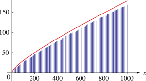
►►►Figure 6.16.2: The logarithmic integral , together with vertical bars indicating the value of for .
Magnify
 ►
►


