SL(2,Z) bilinear transformation

♦ 31—40 of 814 matching pages ♦

(0.004 seconds)

31—40 of 814 matching pages

31: 16.6 Transformations of Variable

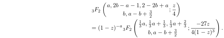
§16.6 Transformations of Variable

►

Quadratic

… ►

Cubic

►

16.6.2

{{}_{3}F_{2}}\left({a,2b-a-1,2-2b+a\atop b,a-b+\frac{3}{2}};\frac{z}{4}\right)% =(1-z)^{-a}{{}_{3}F_{2}}\left({\frac{1}{3}a,\frac{1}{3}a+\frac{1}{3},\frac{1}{% 3}a+\frac{2}{3}\atop b,a-b+\frac{3}{2}};\frac{-27z}{4(1-z)^{3}}\right).

ⓘ

Symbols:: ${{}_{\NVar{p}}F_{\NVar{q}}}\left(\NVar{a_{1},\dots,a_{p}};\NVar{b_{1},\dots,b_% {q}};\NVar{z}\right)$ or ${{}_{\NVar{p}}F_{\NVar{q}}}\left({\NVar{a_{1},\dots,a_{p}}\atop\NVar{b_{1},% \dots,b_{q}}};\NVar{z}\right)$ : alternatively ${{}_{\NVar{p}}F_{\NVar{q}}}\left(\NVar{\mathbf{a}};\NVar{\mathbf{b}};\NVar{z}\right)$ or ${{}_{\NVar{p}}F_{\NVar{q}}}\left({\NVar{\mathbf{a}}\atop\NVar{\mathbf{b}}};% \NVar{z}\right)$
generalized hypergeometric function, $z$ : complex variable, $a,a_{1},\ldots,a_{p}$ : real or complex parameters and $b,b_{1},\ldots,b_{q}$ : real or complex parameters
Referenced by:: §16.6
Permalink:: http://dlmf.nist.gov/16.6.E2
Encodings:: pMML, png, TeX
See also:: Annotations for §16.6, §16.6 and Ch.16

►For Kummer-type transformations of

{{}_{2}F_{2}}

functions see Miller (2003) and Paris (2005a), and for further transformations see Erdélyi et al. (1953a, §4.5), Miller and Paris (2011), Choi and Rathie (2013) and Wang and Rathie (2013).

32: 17.18 Methods of Computation

§17.18 Methods of Computation

… ►The two main methods for computing basic hypergeometric functions are: (1) numerical summation of the defining series given in §§17.4(i) and 17.4(ii); (2) modular transformations. …Method (2) is very powerful when applicable (Andrews (1976, Chapter 5)); however, it is applicable only rarely. Lehner (1941) uses Method (2) in connection with the Rogers–Ramanujan identities. …

33: 14.31 Other Applications

… ►

§14.31(ii) Conical Functions

►The conical functions

\mathsf{P}^{m}_{-\frac{1}{2}+i\tau}\left(x\right)

appear in boundary-value problems for the Laplace equation in toroidal coordinates (§14.19(i)) for regions bounded by cones, by two intersecting spheres, or by one or two confocal hyperboloids of revolution (Kölbig (1981)). These functions are also used in the Mehler–Fock integral transform (§14.20(vi)) for problems in potential and heat theory, and in elementary particle physics (Sneddon (1972, Chapter 7) and Braaksma and Meulenbeld (1967)). The conical functions and Mehler–Fock transform generalize to Jacobi functions and the Jacobi transform; see Koornwinder (1984a) and references therein. …

34: 10.25 Definitions

… ►

10.25.1

z^{2}\frac{{\mathrm{d}}^{2}w}{{\mathrm{d}z}^{2}}+z\frac{\mathrm{d}w}{\mathrm{d% }z}-(z^{2}+\nu^{2})w=0.

ⓘ

Symbols:: $\frac{\mathrm{d}\NVar{f}}{\mathrm{d}\NVar{x}}$ : derivative of $f$ with respect to $x$ , $z$ : complex variable and $\nu$ : complex parameter
A&S Ref:: 9.6.1
Referenced by:: §10.25(ii), §10.25(iii), §10.27, §10.45, §10.74(ii)
Permalink:: http://dlmf.nist.gov/10.25.E1
Encodings:: pMML, png, TeX
See also:: Annotations for §10.25(i), §10.25 and Ch.10

… ►In particular, the principal branch of

I_{\nu}\left(z\right)

is defined in a similar way: it corresponds to the principal value of

(\tfrac{1}{2}z)^{\nu}

, is analytic in

\mathbb{C}\setminus(-\infty,0]

, and two-valued and discontinuous on the cut

\operatorname{ph}z=\pm\pi

. … ►as

z\to\infty

|\operatorname{ph}z|\leq\tfrac{3}{2}\pi-\delta

(<\tfrac{3}{2}\pi)

. … ►

Symbol $\mathscr{Z}_{\nu}\left(z\right)$

►Corresponding to the symbol

\mathscr{C}_{\nu}

introduced in §10.2(ii), we sometimes use

\mathscr{Z}_{\nu}\left(z\right)

to denote

I_{\nu}\left(z\right)

e^{\nu\pi i}K_{\nu}\left(z\right)

, or any nontrivial linear combination of these functions, the coefficients in which are independent of

z

and

\nu

. …

35: 22.21 Tables

… ►Curtis (1964b) tabulates

\operatorname{sn}\left(mK/n,k\right)

\operatorname{cn}\left(mK/n,k\right)

\operatorname{dn}\left(mK/n,k\right)

for

n=2(1)15

m=1(1)n-1

, and

q

(not

k

)

=0(.005)0.35

to 20D. ►Lawden (1989, pp. 280–284 and 293–297) tabulates

\operatorname{sn}\left(x,k\right)

\operatorname{cn}\left(x,k\right)

\operatorname{dn}\left(x,k\right)

\mathcal{E}\left(x,k\right)

\mathrm{Z}\left(x|k\right)

to 5D for

k=0.1(.1)0.9

x=0(.1)X

, where

X

ranges from 1. 5 to 2. 2. … ►Zhang and Jin (1996, p. 678) tabulates

\operatorname{sn}\left(Kx,k\right)

\operatorname{cn}\left(Kx,k\right)

\operatorname{dn}\left(Kx,k\right)

for

k=\frac{1}{4},\frac{1}{2}

and

x=0(.1)4

to 7D. …

36: 32.7 Bäcklund Transformations

… ►Then the transformations …

\mbox{P}_{\mbox{\scriptsize II}}

also has the special transformation … ►The transformations

\mathcal{S}_{j}

, for

j=1,2,3

, generate a group of order 24. … ►The quartic transformation … ►

37: 3.9 Acceleration of Convergence

… ►

§3.9(i) Sequence Transformations

… ►

§3.9(iv) Shanks’ Transformation

►Shanks’ transformation is a generalization of Aitken’s

\Delta^{2}

-process. …Then the transformation of the sequence

\{s_{n}\}

into a sequence

\{t_{n,2k}\}

is given by … ►In Table 3.9.1 values of the transforms

t_{n,2k}

are supplied for …

38: 35.1 Special Notation

… ► ►►►►

$a, b$	complex variables.
…
$\mathbf{Z}$	complex symmetric matrix.
…
$Z_{\kappa}\left(\mathbf{T}\right)$	zonal polynomials.

►The main functions treated in this chapter are the multivariate gamma and beta functions, respectively

\Gamma_{m}\left(a\right)

and

\mathrm{B}_{m}\left(a,b\right)

, and the special functions of matrix argument: Bessel (of the first kind)

A_{\nu}\left(\mathbf{T}\right)

and (of the second kind)

B_{\nu}\left(\mathbf{T}\right)

; confluent hypergeometric (of the first kind)

{{}_{1}F_{1}}\left(a;b;\mathbf{T}\right)

\displaystyle{{}_{1}F_{1}}\left({a\atop b};\mathbf{T}\right)

and (of the second kind)

\Psi\left(a;b;\mathbf{T}\right)

; Gaussian hypergeometric

{{}_{2}F_{1}}\left(a_{1},a_{2};b;\mathbf{T}\right)

\displaystyle{{}_{2}F_{1}}\left({a_{1},a_{2}\atop b};\mathbf{T}\right)

; generalized hypergeometric

{{}_{p}F_{q}}\left(a_{1},\dots,a_{p};b_{1},\dots,b_{q};\mathbf{T}\right)

\displaystyle{{}_{p}F_{q}}\left({a_{1},\dots,a_{p}\atop b_{1},\dots,b_{q}};% \mathbf{T}\right)

. ►An alternative notation for the multivariate gamma function is

\Pi_{m}(a)=\Gamma_{m}\left(a+\tfrac{1}{2}(m+1)\right)

(Herz (1955, p. 480)). Related notations for the Bessel functions are

\mathcal{J}_{\nu+\frac{1}{2}(m+1)}(\mathbf{T})=A_{\nu}\left(\mathbf{T}\right)/% A_{\nu}\left(\boldsymbol{{0}}\right)

(Faraut and Korányi (1994, pp. 320–329)),

K_{m}(0,\dots,0,\nu\mathpunct{|}\mathbf{S},\mathbf{T})=\left|\mathbf{T}\right|% ^{\nu}B_{\nu}\left(\mathbf{S}\mathbf{T}\right)

(Terras (1988, pp. 49–64)), and

\mathcal{K}_{\nu}(\mathbf{T})=\left|\mathbf{T}\right|^{\nu}B_{\nu}\left(% \mathbf{S}\mathbf{T}\right)

(Faraut and Korányi (1994, pp. 357–358)).

39: 10.66 Expansions in Series of Bessel Functions

… ►

10.66.1

\operatorname{ber}_{\nu}x+i\operatorname{bei}_{\nu}x=\sum_{k=0}^{\infty}\frac{% e^{(3\nu+k)\pi i/4}x^{k}J_{\nu+k}\left(x\right)}{2^{k/2}k!}=\sum_{k=0}^{\infty% }\frac{e^{(3\nu+3k)\pi i/4}x^{k}I_{\nu+k}\left(x\right)}{2^{k/2}k!}.

ⓘ

Symbols:: $J_{\NVar{\nu}}\left(\NVar{z}\right)$ : Bessel function of the first kind, $\operatorname{bei}_{\NVar{\nu}}\left(\NVar{x}\right)$ : Kelvin function, $\operatorname{ber}_{\NVar{\nu}}\left(\NVar{x}\right)$ : Kelvin function, $\pi$ : the ratio of the circumference of a circle to its diameter, $\mathrm{e}$ : base of natural logarithm, $!$ : factorial (as in $n!$ ), $\mathrm{i}$ : imaginary unit, $I_{\NVar{\nu}}\left(\NVar{z}\right)$ : modified Bessel function of the first kind, $k$ : nonnegative integer, $x$ : real variable and $\nu$ : complex parameter
A&S Ref:: 9.9.32
Referenced by:: §10.66
Permalink:: http://dlmf.nist.gov/10.66.E1
Encodings:: pMML, png, TeX
See also:: Annotations for §10.66 and Ch.10

►

\operatorname{ber}_{n}\left(x\sqrt{2}\right)=\sum_{k=-\infty}^{\infty}(-1)^{n+% k}J_{n+2k}\left(x\right)I_{2k}\left(x\right),

►

\operatorname{bei}_{n}\left(x\sqrt{2}\right)=\sum_{k=-\infty}^{\infty}(-1)^{n+% k}J_{n+2k+1}\left(x\right)I_{2k+1}\left(x\right).

40: 22.1 Special Notation

… ► ►►►

$x, y$	real variables.
…
$k^{\prime}$	complementary modulus, $k^{2}+{k^{\prime}}^{2}=1$ . If $k\in[0,1]$ , then $k^{\prime}\in[0,1]$ .
…

… ►The functions treated in this chapter are the three principal Jacobian elliptic functions

\operatorname{sn}\left(z,k\right)

\operatorname{cn}\left(z,k\right)

\operatorname{dn}\left(z,k\right)

; the nine subsidiary Jacobian elliptic functions

\operatorname{cd}\left(z,k\right)

\operatorname{sd}\left(z,k\right)

\operatorname{nd}\left(z,k\right)

\operatorname{dc}\left(z,k\right)

\operatorname{nc}\left(z,k\right)

\operatorname{sc}\left(z,k\right)

\operatorname{ns}\left(z,k\right)

\operatorname{ds}\left(z,k\right)

\operatorname{cs}\left(z,k\right)

; the amplitude function

\operatorname{am}\left(x,k\right)

; Jacobi’s epsilon and zeta functions

\mathcal{E}\left(x,k\right)

and

\mathrm{Z}\left(x|k\right)

. … ►Other notations for

\operatorname{sn}\left(z,k\right)

are

\mathrm{sn}(z\mathpunct{|}m)

and

\mathrm{sn}(z,m)

with

m=k^{2}

; see Abramowitz and Stegun (1964) and Walker (1996). …