L%E2%80%99H%C3%B4pital%20rule%20for%20derivatives

SearchAdvancedHelp

(0.004 seconds)

21—30 of 467 matching pages

21: Bibliography

… ►

Algorithm 683: A portable FORTRAN subroutine for exponential integrals of a complex argument. ACM Trans. Math. Software 16 (2), pp. 178–182.

ⓘ

Notes:

Double- and single-precision Fortran, maximum accuracy 18S or 14S.

External Links:

ISSN 0098-3500, Document, GAMS (module 683; package TOMS), MathReview, ZentralBlatt

Referenced by:

1st item, 1st item.

Encodings:

BibTeX

… ►

Applications of basic hypergeometric functions. SIAM Rev. 16 (4), pp. 441–484.

ⓘ

External Links:

Document, MathReview (L. J. Slater), ZentralBlatt

Referenced by:

§17.16, Ch.17.

Encodings:

BibTeX

… ►

Derivatives and integrals with respect to the order of the Struve functions ${𝐇}_{\nu }(x)$ and ${𝐋}_{\nu }(x)$ . J. Math. Anal. Appl. 137 (1), pp. 17–36.

ⓘ

External Links:

ISSN 0022-247X, Document, MathReview (A. McD. Mercer), ZentralBlatt

Referenced by:

§11.4(vi), §11.7(iv).

Encodings:

BibTeX

… ►

Note on the trivial zeros of Dirichlet $L$-functions. Proc. Amer. Math. Soc. 94 (1), pp. 29–30.

ⓘ

External Links:

ISSN 0002-9939, FullText, MathReview (Jerzy Kaczorowski), ZentralBlatt

Referenced by:

(25.15.7), (25.15.8), §25.15(ii), §25.15.

Encodings:

BibTeX

… ►

Quadratic differentials and asymptotics of Laguerre polynomials with varying complex parameters. J. Math. Anal. Appl. 416 (1), pp. 52–80.

ⓘ

External Links:

ISSN 0022-247X, Document, Link, MathReview (Vivek Sahai), ZentralBlatt

Referenced by:

§18.15(vi), §18.15(vi).

Encodings:

BibTeX

…

22: 18.6 Symmetry, Special Values, and Limits to Monomials

… ►

18.6.1 $$L_n^{(\alpha )}\left(0\right)=\frac{{\left(\alpha +1\right)}_n}{n!}.$$

ⓘ

Symbols:

$L_n^{(\alpha )}\left(x\right)$: Laguerre (or generalized Laguerre) polynomial, ${\left(a\right)}_n$: Pochhammer’s symbol (or shifted factorial), $!$: factorial (as in $n!$) and $n$: nonnegative integer

A&S Ref:

22.4.7 (see column for $f_n(0)$)

Referenced by:

§18.17(i), §18.6(i), §18.6(ii)

Permalink:

http://dlmf.nist.gov/18.6.E1

Encodings:

pMML, png, TeX

See also:

Annotations for §18.6(i), §18.6(i), §18.6 and Ch.18

►

Table 18.6.1: Classical OP’s: symmetry and special values.

► ►►►

$p_n(x)$	$p_n(-x)$	$p_n(1)$	$p_{2n}(0)$	$p_{2n+1}^{\prime }(0)$
…
$H_n\left(x\right)$	${(-1)}^n{H}_n\left(x\right)$		${(-1)}^n{\left(n+1\right)}_n$	$2{(-1)}^n{\left(n+1\right)}_{n+1}$
…

►

… ►

18.6.5 $$\underset{\alpha \to \mathrm{\infty }}{lim}\frac{L_n^{(\alpha )}\left(\alpha x\right)}{L_n^{(\alpha )}\left(0\right)}={(1-x)}^n.$$

ⓘ

Symbols:

$L_n^{(\alpha )}\left(x\right)$: Laguerre (or generalized Laguerre) polynomial, $n$: nonnegative integer and $x$: real variable

Referenced by:

§18.6(ii)

Permalink:

http://dlmf.nist.gov/18.6.E5

Encodings:

pMML, png, TeX

See also:

Annotations for §18.6(ii), §18.6 and Ch.18

23: 18.9 Recurrence Relations and Derivatives

§18.9 Recurrence Relations and Derivatives

… ►

Jacobi

… ►

Ultraspherical

… ►

Laguerre

… ►

Hermite

…

24: 29.1 Special Notation

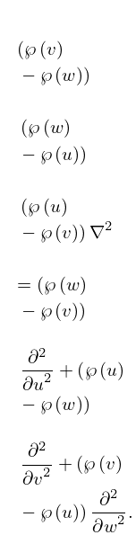
… ►All derivatives are denoted by differentials, not by primes. … ►The relation to the Lamé functions $L_{c\nu }^{(m)}$, $L_{s\nu }^{(m)}$of Jansen (1977) is given by ►

$${\mathrm{𝐸𝑐}}_{\nu }^{2m}(z,k^2)={(-1)}^m{L}_{c\nu }^{(2m)}(\psi ,k_{}^{\prime }{}_{}{}^2),$$

►

$${\mathrm{𝐸𝑐}}_{\nu }^{2m+1}(z,k^2)={(-1)}^m{L}_{s\nu }^{(2m+1)}(\psi ,k_{}^{\prime }{}_{}{}^2),$$

►

$${\mathrm{𝐸𝑠}}_{\nu }^{2m+1}(z,k^2)={(-1)}^m{L}_{c\nu }^{(2m+1)}(\psi ,k_{}^{\prime }{}_{}{}^2),$$

…

25: 18.1 Notation

… ►

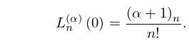
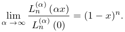
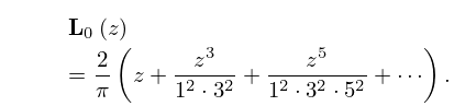
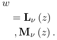
Laguerre: $L_n^{(\alpha )}\left(x\right)$ and $L_n\left(x\right)=L_n^{(0)}\left(x\right)$. ($L_n^{(\alpha )}\left(x\right)$ with $\alpha \ne 0$ is also called Generalized Laguerre.)

►

Hermite: $H_n\left(x\right)$, ${\mathrm{𝐻𝑒}}_n\left(x\right)$.

… ►

$q$-Laguerre: $L_n^{(\alpha )}(x;q)$.

… ►

Continuous $q$-Hermite: $H_n\left(x|q\right)$.

…

26: 11.2 Definitions

… ►

11.2.2 $${𝐋}_{\nu }\left(z\right)=-\mathrm{i}{\mathrm{e}}^{-\frac{1}{2}\pi \mathrm{i}\nu }{𝐇}_{\nu }\left(\mathrm{i}z\right)={(\frac{1}{2}z)}^{\nu +1}\sum _{n=0}^{\mathrm{\infty }}\frac{{(\frac{1}{2}z)}^{2n}}{\mathrm{\Gamma }\left(n+\frac{3}{2}\right)\mathrm{\Gamma }\left(n+\nu +\frac{3}{2}\right)}.$$

ⓘ

Defines:

${𝐋}_{\nu }\left(z\right)$: modified Struve function

Symbols:

$\mathrm{\Gamma }\left(z\right)$: gamma function, ${𝐇}_{\nu }\left(z\right)$: Struve function, $\pi$: the ratio of the circumference of a circle to its diameter, $\mathrm{e}$: base of natural logarithm, $\mathrm{i}$: imaginary unit, $z$: complex variable, $\nu$: real or complex order and $n$: integer order

A&S Ref:

12.2.1

Referenced by:

§11.13(ii), §11.2(i), §11.4(i), §11.4(iii), §11.5(ii), §11.5(i), §11.6(ii), §11.6(ii)

Permalink:

http://dlmf.nist.gov/11.2.E2

Encodings:

pMML, png, TeX

See also:

Annotations for §11.2(i), §11.2 and Ch.11

… ►The functions $z^{-\nu -1}{𝐇}_{\nu }\left(z\right)$ and $z^{-\nu -1}{𝐋}_{\nu }\left(z\right)$ are entire functions of $z$ and $\nu$. … ►

11.2.4 $${𝐋}_0\left(z\right)=\frac{2}{\pi }\left(z+\frac{z^3}{1^2\cdot 3^2}+\frac{z^5}{1^2\cdot 3^2\cdot 5^2}+\mathrm{\cdots }\right).$$

ⓘ

Symbols:

$\pi$: the ratio of the circumference of a circle to its diameter, ${𝐋}_{\nu }\left(z\right)$: modified Struve function and $z$: complex variable

Permalink:

http://dlmf.nist.gov/11.2.E4

Encodings:

pMML, png, TeX

See also:

Annotations for §11.2(i), §11.2 and Ch.11

… ►Unless indicated otherwise, ${𝐇}_{\nu }\left(z\right)$, ${𝐊}_{\nu }\left(z\right)$, ${𝐋}_{\nu }\left(z\right)$, and ${𝐌}_{\nu }\left(z\right)$ assume their principal values throughout the DLMF. … ►

11.2.10 $$w={𝐋}_{\nu }\left(z\right),{𝐌}_{\nu }\left(z\right).$$

ⓘ

Symbols:

${𝐌}_{\nu }\left(z\right)$: modified Struve function, ${𝐋}_{\nu }\left(z\right)$: modified Struve function, $z$: complex variable and $\nu$: real or complex order

Permalink:

http://dlmf.nist.gov/11.2.E10

Encodings:

pMML, png, TeX

See also:

Annotations for §11.2(ii), §11.2(ii), §11.2 and Ch.11

…

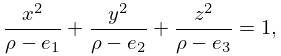
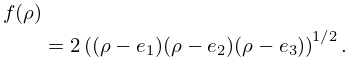
27: 23.19 Interrelations

… ►

23.19.1 $$\lambda \left(\tau \right)=16{\left(\frac{{\eta }^2\left(2\tau \right)\eta \left(\frac{1}{2}\tau \right)}{{\eta }^3\left(\tau \right)}\right)}^8,$$

ⓘ

Symbols:

$\eta \left(\tau \right)$: Dedekind’s eta function (or Dedekind modular function), $\lambda \left(\tau \right)$: elliptic modular function and $\tau$: complex variable

Permalink:

http://dlmf.nist.gov/23.19.E1

Encodings:

pMML, png, TeX

See also:

Annotations for §23.19 and Ch.23

… ►

23.19.3 $$J\left(\tau \right)=\frac{g_2^3}{g_2^3-27g_3^2},$$

ⓘ

Symbols:

$J\left(\tau \right)$: Klein’s complete invariant, $g_j$: Weierstrass lattice invariants $g_2$, $g_3$ , $𝕃$: lattice and $\tau$: complex variable

Permalink:

http://dlmf.nist.gov/23.19.E3

Encodings:

pMML, png, TeX

See also:

Annotations for §23.19 and Ch.23

►where $g_2,g_3$ are the invariants of the lattice $𝕃$ with generators $1$ and $\tau$; see §23.3(i). … ►

23.19.4 $$\mathrm{\Delta }={(2\pi )}^{12}{\eta }^{24}\left(\tau \right).$$

ⓘ

Symbols:

$\eta \left(\tau \right)$: Dedekind’s eta function (or Dedekind modular function), $\pi$: the ratio of the circumference of a circle to its diameter, $\mathrm{\Delta }$: discriminant and $\tau$: complex variable

Referenced by:

§23.19

Permalink:

http://dlmf.nist.gov/23.19.E4

Encodings:

pMML, png, TeX

See also:

Annotations for §23.19 and Ch.23

28: 11.7 Integrals and Sums

… ►

11.7.3 $$\int z^{\nu }{𝐋}_{\nu -1}\left(z\right)dz=z^{\nu }{𝐋}_{\nu }\left(z\right),$$

ⓘ

Symbols:

$dx$: differential of $x$ , $\int$: integral, ${𝐋}_{\nu }\left(z\right)$: modified Struve function, $z$: complex variable and $\nu$: real or complex order

Permalink:

http://dlmf.nist.gov/11.7.E3

Encodings:

pMML, png, TeX

See also:

Annotations for §11.7(i), §11.7 and Ch.11

►

11.7.4 $$\int z^{-\nu }{𝐋}_{\nu +1}\left(z\right)dz=z^{-\nu }{𝐋}_{\nu }\left(z\right)-\frac{2^{-\nu }z}{\sqrt{\pi }\mathrm{\Gamma }\left(\nu +\frac{3}{2}\right)}.$$

ⓘ

Symbols:

$\mathrm{\Gamma }\left(z\right)$: gamma function, $\pi$: the ratio of the circumference of a circle to its diameter, $dx$: differential of $x$ , $\int$: integral, ${𝐋}_{\nu }\left(z\right)$: modified Struve function, $z$: complex variable and $\nu$: real or complex order

Permalink:

http://dlmf.nist.gov/11.7.E4

Encodings:

pMML, png, TeX

See also:

Annotations for §11.7(i), §11.7 and Ch.11

… ►The following Laplace transforms of ${𝐇}_{\nu }\left(t\right)$ require $\mathrm{\Re }a>0$ for convergence, while those of ${𝐋}_{\nu }\left(t\right)$ require $\mathrm{\Re }a>1$. … ►

${\displaystyle {\int }_0^{\mathrm{\infty }}}{\mathrm{e}}^{-at}{𝐋}_1\left(t\right)dt$

… ►For integrals of ${𝐇}_{\nu }\left(x\right)$ and ${𝐋}_{\nu }\left(x\right)$ with respect to the order $\nu$, see Apelblat (1989). …

29: 11.13 Methods of Computation

… ►For a review of methods for the computation of ${𝐇}_{\nu }\left(z\right)$ see Zanovello (1975). For simple and effective approximations to ${𝐇}_0\left(z\right)$ and ${𝐇}_1\left(z\right)$ see Aarts and Janssen (2016). … ►Subsequently ${𝐇}_{\nu }\left(z\right)$ and ${𝐋}_{\nu }\left(z\right)$ are obtainable via (11.2.5) and (11.2.6). … ►Then from the limiting forms for small argument (§§11.2(i), 10.7(i), 10.30(i)), limiting forms for large argument (§§11.6(i), 10.7(ii), 10.30(ii)), and the connection formulas (11.2.5) and (11.2.6), it is seen that ${𝐇}_{\nu }\left(x\right)$ and ${𝐋}_{\nu }\left(x\right)$ can be computed in a stable manner by integrating forwards, that is, from the origin toward infinity. … ►Sequences of values of ${𝐇}_{\nu }\left(z\right)$ and ${𝐋}_{\nu }\left(z\right)$, with $z$ fixed, can be computed by application of the inhomogeneous difference equations (11.4.23) and (11.4.25). …

30: 23.21 Physical Applications

… ►

23.21.1 $$\frac{x^2}{\rho -e_1}+\frac{y^2}{\rho -e_2}+\frac{z^2}{\rho -e_3}=1,$$

ⓘ

Symbols:

$e_j$: Weierstrass lattice roots, $𝕃$: lattice, $x$: real part of $z$ , $y$: imaginary part of $z$ , $z$: complex and $\rho$: roots

Permalink:

http://dlmf.nist.gov/23.21.E1

Encodings:

pMML, png, TeX

See also:

Annotations for §23.21(iii), §23.21 and Ch.23

… ►

23.21.2 $$(\eta -\zeta )(\zeta -\xi )(\xi -\eta ){\nabla }^2=(\zeta -\eta )f(\xi )f^{\prime }(\xi )\frac{\partial }{\partial \xi }+(\xi -\zeta )f(\eta )f^{\prime }(\eta )\frac{\partial }{\partial \eta }+(\eta -\xi )f(\zeta )f^{\prime }(\zeta )\frac{\partial }{\partial \zeta },$$

ⓘ

Symbols:

$\frac{\partial f}{\partial x}$: partial derivative of $f$ with respect to $x$ , $\partial x$: partial differential of $x$ , $\xi$: ellipsoidal coordinate, $\eta$: ellipsoidal coordinate, $\zeta$: ellipsoidal coordinate and $f(\rho )$: function

Permalink:

http://dlmf.nist.gov/23.21.E2

Encodings:

pMML, png, TeX

See also:

Annotations for §23.21(iii), §23.21 and Ch.23

… ►

23.21.3 $$f(\rho )=2{\left((\rho -e_1)(\rho -e_2)(\rho -e_3)\right)}^{1/2}.$$

ⓘ

Symbols:

$e_j$: Weierstrass lattice roots, $𝕃$: lattice, $\rho$: roots and $f(\rho )$: function

Permalink:

http://dlmf.nist.gov/23.21.E3

Encodings:

pMML, png, TeX

See also:

Annotations for §23.21(iii), §23.21 and Ch.23

… ►

23.21.5 $$\left(\mathrm{\wp }\left(v\right)-\mathrm{\wp }\left(w\right)\right)\left(\mathrm{\wp }\left(w\right)-\mathrm{\wp }\left(u\right)\right)\left(\mathrm{\wp }\left(u\right)-\mathrm{\wp }\left(v\right)\right){\nabla }^2=\left(\mathrm{\wp }\left(w\right)-\mathrm{\wp }\left(v\right)\right)\frac{{\partial }^2}{{\partial u}^2}+\left(\mathrm{\wp }\left(u\right)-\mathrm{\wp }\left(w\right)\right)\frac{{\partial }^2}{{\partial v}^2}+\left(\mathrm{\wp }\left(v\right)-\mathrm{\wp }\left(u\right)\right)\frac{{\partial }^2}{{\partial w}^2}.$$

ⓘ

Symbols:

$\mathrm{\wp }\left(z\right)$ (= $\mathrm{\wp }\left(z|𝕃\right)$ = $\mathrm{\wp }(z;g_2,g_3)$): Weierstrass $\mathrm{\wp }$-function, $\frac{\partial f}{\partial x}$: partial derivative of $f$ with respect to $x$ , $\partial x$: partial differential of $x$ , $𝕃$: lattice, $u$: change of variable, $v$: change of variable and $w$: change of variable

Permalink:

http://dlmf.nist.gov/23.21.E5

Encodings:

pMML, png, TeX

See also:

Annotations for §23.21(iii), §23.21 and Ch.23

…