Hermite polynomials

SearchAdvancedHelp

(0.006 seconds)

31—40 of 59 matching pages

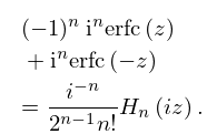
31: 7.18 Repeated Integrals of the Complementary Error Function

… ►

Hermite Polynomials

►

7.18.8 $${(-1)}^n{\mathrm{i}}^n\mathrm{erfc}\left(z\right)+{\mathrm{i}}^n\mathrm{erfc}\left(-z\right)=\frac{{\mathrm{i}}^{-n}}{2^{n-1}n!}{H}_n\left(\mathrm{i}z\right).$$

ⓘ

Symbols:

$H_n\left(x\right)$: Hermite polynomial, $!$: factorial (as in $n!$), $\mathrm{i}$: imaginary unit, ${\mathrm{i}}^n\mathrm{erfc}\left(z\right)$: repeated integrals of the complementary error function, $z$: complex variable and $n$: nonnegative integer

A&S Ref:

7.2.11

Permalink:

http://dlmf.nist.gov/7.18.E8

Encodings:

pMML, png, TeX

See also:

Annotations for §7.18(iv), §7.18(iv), §7.18 and Ch.7

…

32: 18.39 Applications in the Physical Sciences

… ►

${\psi }_n(x)={\left(c{h}_n\right)}^{-1/2}{w}^{1/2}(cx)H_n\left(cx\right),$

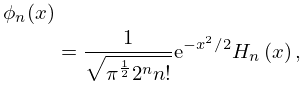
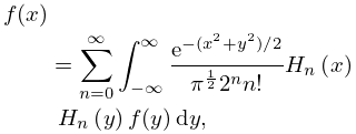
… ►Here the $H_n\left(x\right)$ are Hermite polynomials, $w(x)={\mathrm{e}}^{-x^2}$, and $h_n=2^{n}n!\sqrt{\pi }$. … ►

18.39.20 $${\widehat{\psi }}_{n+3}(x)=\sqrt{w(x)}{\widehat{H}}_{n+3}\left(x\right),$$ $n=-3,0,1,2,\mathrm{\dots }$,

ⓘ

Symbols:

${\widehat{H}}_n\left(x\right)$: exceptional Hermite polynomial, $w(x)$: weight function, $n$: nonnegative integer and $x$: real variable

Permalink:

http://dlmf.nist.gov/18.39.E20

Encodings:

pMML, png, TeX

See also:

Annotations for §18.39(i), §18.39(i), §18.39 and Ch.18

►and eigenvalues $n+3$, with $n$ as above, with $w(x)$ the weight function of (18.36.10), and ${\widehat{H}}_{n+3}\left(x\right)$ a type III Hermite EOP defined by (18.36.8) and (18.36.9). … ►This seems odd at first glance as ${\widehat{H}}_{n+3}\left(x\right)$ is a polynomial of order $n+3$ for $n=0,1,2,\mathrm{\dots }$, seemingly suggesting that for $n=0$, this being the first excited state, i. …

33: 1.17 Integral and Series Representations of the Dirac Delta

… ►

Hermite Polynomials (§18.3)

►

1.17.24 $$\delta \left(x-a\right)=\frac{{\mathrm{e}}^{-(x^2+a^2)/2}}{\sqrt{\pi }}\sum _{k=0}^{\mathrm{\infty }}\frac{H_k\left(x\right)H_k\left(a\right)}{2^{k}k!}.$$

ⓘ

Symbols:

$\delta \left(x-a\right)$: Dirac delta (or Dirac delta function), $H_n\left(x\right)$: Hermite polynomial, $\pi$: the ratio of the circumference of a circle to its diameter, $\mathrm{e}$: base of natural logarithm, $!$: factorial (as in $n!$) and $k$: integer

Referenced by:

§1.17(iii), §1.17(iv)

Permalink:

http://dlmf.nist.gov/1.17.E24

Encodings:

pMML, png, TeX

See also:

Annotations for §1.17(iii), §1.17(iii), §1.17 and Ch.1

…

34: 18.29 Asymptotic Approximations for $q$-Hahn and Askey–Wilson Classes

… ►For a uniform asymptotic expansion of the Stieltjes–Wigert polynomials, see Wang and Wong (2006). ►For asymptotic approximations to the largest zeros of the $q$-Laguerre and continuous $q^{-1}$-Hermite polynomials see Chen and Ismail (1998).

35: 18.15 Asymptotic Approximations

… ►

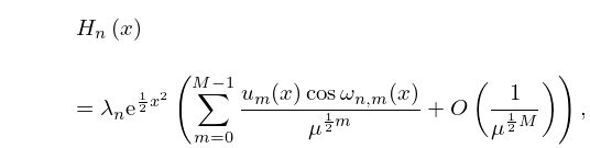
§18.15(v) Hermite

… ►

18.15.27 $$H_n\left(x\right)={\lambda }_n{\mathrm{e}}^{\frac{1}{2}{x}^2}\left(\sum _{m=0}^{M-1}\frac{u_m(x)\cos {\omega }_{n,m}(x)}{{\mu }^{\frac{1}{2}m}}+O\left(\frac{1}{{\mu }^{\frac{1}{2}M}}\right)\right),$$

ⓘ

Symbols:

$O\left(x\right)$: order not exceeding, $H_n\left(x\right)$: Hermite polynomial, $\cos z$: cosine function, $\mathrm{e}$: base of natural logarithm, $m$: nonnegative integer, $n$: nonnegative integer, ${\omega }_{n,m}(x)$ and $x$: real variable

Permalink:

http://dlmf.nist.gov/18.15.E27

Encodings:

pMML, png, TeX

See also:

Annotations for §18.15(v), §18.15 and Ch.18

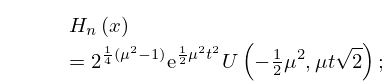
… ►With $\mu =\sqrt{2n+1}$ the expansions in Chapter 12 are for the parabolic cylinder function $U(-\frac{1}{2}{\mu }^2,\mu t\sqrt{2})$, which is related to the Hermite polynomials via ►

18.15.28 $$H_n\left(x\right)=2^{\frac{1}{4}({\mu }^2-1)}{\mathrm{e}}^{\frac{1}{2}{\mu }^2{t}^2}U(-\frac{1}{2}{\mu }^2,\mu t\sqrt{2});$$

ⓘ

Symbols:

$H_n\left(x\right)$: Hermite polynomial, $\mathrm{e}$: base of natural logarithm, $U(a,z)$: parabolic cylinder function, $t$: real variable, $n$: nonnegative integer and $x$: real variable

Permalink:

http://dlmf.nist.gov/18.15.E28

Encodings:

pMML, png, TeX

See also:

Annotations for §18.15(v), §18.15 and Ch.18

… ►For asymptotic approximations of Jacobi, ultraspherical, and Laguerre polynomials in terms of Hermite polynomials, see López and Temme (1999a). …

36: 1.18 Linear Second Order Differential Operators and Eigenfunction Expansions

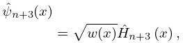
… ►Writing Hermite’s differential equation (see Tables 18.3.1 and 18.8.1) in the form above, the eigenfunctions are ${\mathrm{e}}^{-x^2/2}{H}_n\left(x\right)$ ($H_n$ a Hermite polynomial, $n=0,1,2,\mathrm{\dots }$), with eigenvalues ${\lambda }_n=2n+1\in {𝝈}_p$, for the differential operator … ►

1.18.42 $${\varphi }_n(x)=\frac{1}{\sqrt{{\pi }^{\frac{1}{2}}{2}^{n}n!}}{\mathrm{e}}^{-x^2/2}{H}_n\left(x\right),$$

ⓘ

Symbols:

$H_n\left(x\right)$: Hermite polynomial, $\pi$: the ratio of the circumference of a circle to its diameter, $\mathrm{e}$: base of natural logarithm, $!$: factorial (as in $n!$) and $n$: nonnegative integer

Permalink:

http://dlmf.nist.gov/1.18.E42

Encodings:

pMML, png, TeX

See also:

Annotations for §1.18(v), §1.18(v), §1.18 and Ch.1

… ►

1.18.43 $$f(x)=\sum _{n=0}^{\mathrm{\infty }}{\int }_{-\mathrm{\infty }}^{\mathrm{\infty }}\frac{{\mathrm{e}}^{-(x^2+y^2)/2}}{{\pi }^{\frac{1}{2}}{2}^{n}n!}{H}_n\left(x\right)H_n\left(y\right)f(y)dy,$$

ⓘ

Symbols:

$H_n\left(x\right)$: Hermite polynomial, $\pi$: the ratio of the circumference of a circle to its diameter, $dx$: differential of $x$ , $\mathrm{e}$: base of natural logarithm, $!$: factorial (as in $n!$), $\int$: integral and $n$: nonnegative integer

Permalink:

http://dlmf.nist.gov/1.18.E43

Encodings:

pMML, png, TeX

See also:

Annotations for §1.18(v), §1.18(v), §1.18 and Ch.1

…

37: 3.5 Quadrature

… ►The $p_n(x)$ are the monic Hermite polynomials $H_n\left(x\right)$ (§18.3). ►

Table 3.5.10: Nodes and weights for the 5-point Gauss–Hermite formula.

► ►►

$\pm x_k$		$w_k$
…

►

►

Table 3.5.11: Nodes and weights for the 10-point Gauss–Hermite formula.

► ►►

$\pm x_k$		$w_k$
…

►

►

Table 3.5.12: Nodes and weights for the 15-point Gauss–Hermite formula.

► ►►

$\pm x_k$		$w_k$
…

►

►

Table 3.5.13: Nodes and weights for the 20-point Gauss–Hermite formula.

► ►►

$\pm x_k$		$w_k$
…

►

…

38: 28.8 Asymptotic Expansions for Large $q$

… ►Also let $\xi =2\sqrt{h}\cos x$ and $D_m\left(\xi \right)={\mathrm{e}}^{-{\xi }^2/4}{\mathrm{𝐻𝑒}}_m\left(\xi \right)$ (§18.3). …

39: Bibliography I

… ►

$q$-Hermite polynomials, biorthogonal rational functions, and $q$-beta integrals. Trans. Amer. Math. Soc. 346 (1), pp. 63–116.

ⓘ

External Links:

ISSN 0002-9947, FullText, MathReview (R. A. Askey), ZentralBlatt

Referenced by:

§18.28(vii).

Encodings:

BibTeX

…

40: 29.7 Asymptotic Expansions

… ►Müller (1966a, b) found three formal asymptotic expansions for a fundamental system of solutions of (29.2.1) (and (29.11.1)) as $\nu \to \mathrm{\infty }$, one in terms of Jacobian elliptic functions and two in terms of Hermite polynomials. …