Gegenbauer%20addition%20theorem
(0.001 seconds)
11—20 of 259 matching pages
11: 18.17 Integrals
…
►
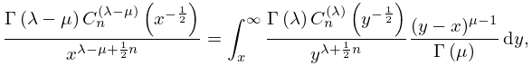
18.17.5
.
…
►For addition formulas corresponding to (18.17.5) and (18.17.6) see (18.18.8) and (18.18.9), respectively.
…
►
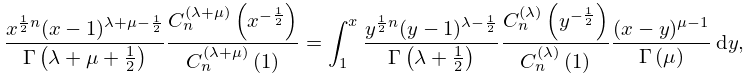
18.17.12
, ,
►
18.17.13
, .
…
►
18.17.16_5
…
12: 1.10 Functions of a Complex Variable
…
►
Picard’s Theorem
… ►In addition, … ►Also, if in addition is analytic at , then … ►and hence , that is (18.9.19). The recurrence relation for in §18.9(i) follows from , and the contour integral representation for in §18.10(iii) is just (1.10.27).13: 18.5 Explicit Representations
…
►
…
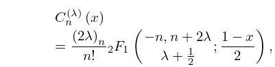
18.5.9
►
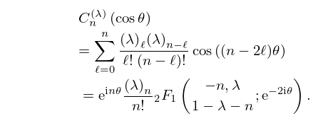
18.5.10
►
18.5.11
…
►Similarly in the cases of the ultraspherical polynomials and the Laguerre polynomials we assume that , and , unless
stated otherwise.
…
►
14: Tom M. Apostol
…
►Apostol was born on August 20, 1923.
…
►In 1998, the Mathematical Association of America (MAA) awarded him the annual Trevor Evans Award, presented to authors of an exceptional article that is accessible to undergraduates, for his piece entitled “What Is the Most Surprising Result in Mathematics?” (Answer: the prime number theorem).
…In addition, he was the co-author of New Horizons in Geometry, published by the MAA, which received the CHOICE “Outstanding Academic Title” award in 2013.
…He additionally served as a visiting lecturer for the MAA, and as a member of the MAA Board of Governors.
…
15: 15.9 Relations to Other Functions
…
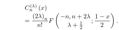
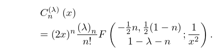
►
Gegenbauer (or Ultraspherical)
►
15.9.2
►
15.9.3
…
►
§15.9(iii) Gegenbauer Function
►This is a generalization of Gegenbauer (or ultraspherical) polynomials (§18.3). …16: 27.15 Chinese Remainder Theorem
§27.15 Chinese Remainder Theorem
… ►This theorem is employed to increase efficiency in calculating with large numbers by making use of smaller numbers in most of the calculation. …Their product has 20 digits, twice the number of digits in the data. By the Chinese remainder theorem each integer in the data can be uniquely represented by its residues (mod ), (mod ), (mod ), and (mod ), respectively. …These numbers, in turn, are combined by the Chinese remainder theorem to obtain the final result , which is correct to 20 digits. …17: 14.28 Sums
…
►
§14.28(i) Addition Theorem
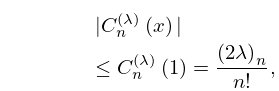
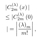
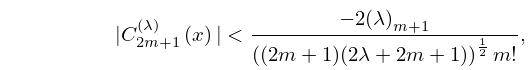
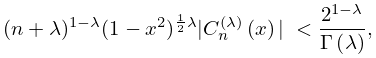
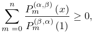
… ►For generalizations in terms of Gegenbauer and Jacobi polynomials, see Theorem 2. 1 in Cohl (2013b) and Theorem 1 in Cohl (2013a) respectively. …18: 18.14 Inequalities
19: 18.3 Definitions
…
►
1.
…
►
Table 18.3.1: Orthogonality properties for classical OP’s: intervals, weight functions, standardizations, leading coefficients, and parameter constraints.
…
►
►
►
…
►In addition to the orthogonal property given by Table 18.3.1, the Chebyshev polynomials , , are orthogonal on the discrete point set comprising the zeros , of :
…
| Name | Constraints | ||||||
|---|---|---|---|---|---|---|---|
| … | |||||||
| Ultraspherical (Gegenbauer) | |||||||
| … | |||||||
20: Errata
…
►
Equation (18.7.25)
…
►
Chapters 14 Legendre and Related Functions, 15 Hypergeometric Function
…
►
Chapters 8, 20, 36
…
►
Table 18.9.1
…
►
References
…
18.7.25
We included the case .
The coefficient for in the first row of this table originally omitted the parentheses and was given as , instead of .
| ⋮ | |||
Reported 2010-09-16 by Kendall Atkinson.
