Gauss–Christoffel quadrature

SearchAdvancedHelp

(0.001 seconds)

1—10 of 141 matching pages

1: 3.5 Quadrature

… ►

§3.5(v) Gauss Quadrature

… ►In Gauss quadrature (also known as Gauss–Christoffel quadrature) we use (3.5.15) with nodes $x_k$ the zeros of $p_n$, and weights $w_k$ given by …The remainder is given by … ►

Gauss–Laguerre Formula

… ►

§3.5(viii) Complex Gauss Quadrature

…

2: Bibliography G

… ►

Stable computation of high order Gauss quadrature rules using discretization for measures in radiation transfer. J. Quant. Spectrosc. Radiat. Transfer 68 (2), pp. 213–223.

ⓘ

Referenced by:

§18.39(iii).

Encodings:

BibTeX

… ►

Algorithm 726: ORTHPOL — a package of routines for generating orthogonal polynomials and Gauss-type quadrature rules. ACM Trans. Math. Software 20 (1), pp. 21–62.

ⓘ

Notes:

For remark see same journal 24(1998), p. 355.

External Links:

Document, ISSN 0098-3500, GAMS (module 726; package TOMS), ZentralBlatt

Referenced by:

2nd item, §3.5(v), §3.5(v).

Encodings:

BibTeX

… ►

Construction of Gauss-Christoffel quadrature formulas. Math. Comp. 22, pp. 251–270.

ⓘ

External Links:

ISSN 0025-5718, Document, Link, MathReview (R. E. Barnhill)

Referenced by:

§18.39(iii).

Encodings:

BibTeX

… ►

Gauss quadrature approximations to hypergeometric and confluent hypergeometric functions. J. Comput. Appl. Math. 139 (1), pp. 173–187.

ⓘ

External Links:

ISSN 0377-0427, Document, MathReview (Hasan Taşeli), ZentralBlatt

Referenced by:

§13.29(iii), §15.19(iii).

Encodings:

BibTeX

… ►

Calculation of Gauss quadrature rules. Math. Comp. 23 (106), pp. 221–230.

ⓘ

Notes:

Loose microfiche suppl. A1–A10

External Links:

FullText, MathReview (F. Stenger), ZentralBlatt

Referenced by:

§18.39(iii), §3.5(vi).

Encodings:

BibTeX

…

3: 35.10 Methods of Computation

… ►Other methods include numerical quadrature applied to double and multiple integral representations. See Yan (1992) for the ${}_1{}^{}F_1^{}$ and ${}_2{}^{}F_1^{}$ functions of matrix argument in the case $m=2$, and Bingham et al. (1992) for Monte Carlo simulation on $𝐎(m)$ applied to a generalization of the integral (35.5.8). …

4: 15.19 Methods of Computation

… ►The Gauss series (15.2.1) converges for . … ►Large values of $|a|$ or $|b|$, for example, delay convergence of the Gauss series, and may also lead to severe cancellation. ►For fast computation of $F(a,b;c;z)$ with $a,b$ and $c$ complex, and with application to Pöschl–Teller–Ginocchio potential wave functions, see Michel and Stoitsov (2008). … ►Gauss quadrature approximations are discussed in Gautschi (2002b). … ►For example, in the half-plane $\mathrm{\Re }z\le \frac{1}{2}$ we can use (15.12.2) or (15.12.3) to compute $F(a,b;c+N+1;z)$ and $F(a,b;c+N;z)$, where $N$ is a large positive integer, and then apply (15.5.18) in the backward direction. …

5: 18.2 General Orthogonal Polynomials

… ►

§18.2(v) Christoffel–Darboux Formula

… ►

18.2.12 $$K_n(x,y)\equiv \sum _{\mathrm{\ell }=0}^n\frac{p_{\mathrm{\ell }}(x)p_{\mathrm{\ell }}(y)}{h_{\mathrm{\ell }}}=\frac{k_n}{h_n{k}_{n+1}}\frac{p_{n+1}(x)p_n(y)-p_n(x)p_{n+1}(y)}{x-y},$$ $x\ne y$,

ⓘ

Symbols:

$\equiv$: equals by definition, $(a,b)$: open interval, $y$: real variable, $p_n(x)$: polynomial of degree $n$ , $\mathrm{\ell }$: nonnegative integer, $n$: nonnegative integer, $x$: real variable, $h_n$ and $k_n$

A&S Ref:

22.12.1

Referenced by:

§18.2(v), Erratum (V1.2.0) for Equations (18.2.12), (18.2.13)

Permalink:

http://dlmf.nist.gov/18.2.E12

Encodings:

pMML, png, TeX

Addition (effective with 1.2.0):

The left-hand side was updated to include the definition of the Christoffel–Darboux kernel $K_n(x,y)$.

See also:

Annotations for §18.2(v), §18.2 and Ch.18

… ►

Confluent Form

… ►For usage of the zeros of an OP in Gauss quadrature see §3.5(v). … ►are the Christoffel numbers, see also (3.5.18). …

6: 18.38 Mathematical Applications

… ►

Quadrature

►Classical OP’s play a fundamental role in Gaussian quadrature. … ►

Quadrature “Extended” to Pseudo-Spectral (DVR) Representations of Operators in One and Many Dimensions

►The basic ideas of Gaussian quadrature, and their extensions to non-classical weight functions, and the computation of the corresponding quadrature abscissas and weights, have led to discrete variable representations, or DVRs, of Sturm–Liouville and other differential operators. … ►For the generalized hypergeometric function ${}_3{}^{}F_2^{}$ see (16.2.1). …

7: 9.17 Methods of Computation

… ►For details, including the application of a generalized form of Gaussian quadrature, see Gordon (1969, Appendix A) and Schulten et al. (1979). … ►The second method is to apply generalized Gauss–Laguerre quadrature (§3.5(v)) to the integral (9.5.8). … ►For quadrature methods for Scorer functions see Gil et al. (2001), Lee (1980), and Gordon (1970, Appendix A); but see also Gautschi (1983). …

8: 15.5 Derivatives and Contiguous Functions

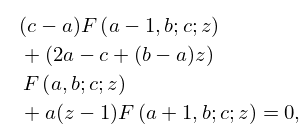
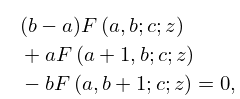
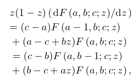
… ►The six functions $F(a\pm 1,b;c;z)$, $F(a,b\pm 1;c;z)$, $F(a,b;c\pm 1;z)$ are said to be contiguous to $F(a,b;c;z)$. ►

15.5.11 $$(c-a)F(a-1,b;c;z)+\left(2a-c+(b-a)z\right)F(a,b;c;z)+a(z-1)F(a+1,b;c;z)=0,$$

ⓘ

Symbols:

$F(a,b;c;z)$ or $F(\genfrac{}{}{0pt}{}{a,b}{c};z)$: $={}_2{}^{}F_1^{}(a,b;c;z)$ Gauss’ hypergeometric function, $z$: complex variable, $a$: real or complex parameter, $b$: real or complex parameter and $c$: real or complex parameter

Referenced by:

§15.4(i), §15.5(ii)

Permalink:

http://dlmf.nist.gov/15.5.E11

Encodings:

pMML, png, TeX

See also:

Annotations for §15.5(ii), §15.5 and Ch.15

►

15.5.12 $$(b-a)F(a,b;c;z)+aF(a+1,b;c;z)-bF(a,b+1;c;z)=0,$$

ⓘ

Symbols:

$F(a,b;c;z)$ or $F(\genfrac{}{}{0pt}{}{a,b}{c};z)$: $={}_2{}^{}F_1^{}(a,b;c;z)$ Gauss’ hypergeometric function, $z$: complex variable, $a$: real or complex parameter, $b$: real or complex parameter and $c$: real or complex parameter

Permalink:

http://dlmf.nist.gov/15.5.E12

Encodings:

pMML, png, TeX

See also:

Annotations for §15.5(ii), §15.5 and Ch.15

… ►By repeated applications of (15.5.11)–(15.5.18) any function $F(a+k,b+\mathrm{\ell };c+m;z)$, in which $k,\mathrm{\ell },m$ are integers, can be expressed as a linear combination of $F(a,b;c;z)$ and any one of its contiguous functions, with coefficients that are rational functions of $a,b,c$, and $z$. … ►

15.5.20 $$z(1-z)\left(dF(a,b;c;z)/dz\right)=(c-a)F(a-1,b;c;z)+(a-c+bz)F(a,b;c;z)=(c-b)F(a,b-1;c;z)+(b-c+az)F(a,b;c;z),$$

ⓘ

Symbols:

$F(a,b;c;z)$ or $F(\genfrac{}{}{0pt}{}{a,b}{c};z)$: $={}_2{}^{}F_1^{}(a,b;c;z)$ Gauss’ hypergeometric function, $\frac{df}{dx}$: derivative of $f$ with respect to $x$ , $z$: complex variable, $a$: real or complex parameter, $b$: real or complex parameter and $c$: real or complex parameter

Permalink:

http://dlmf.nist.gov/15.5.E20

Encodings:

pMML, png, TeX

See also:

Annotations for §15.5(ii), §15.5 and Ch.15

…

9: 6.18 Methods of Computation

… ►Quadrature of the integral representations is another effective method. For example, the Gauss–Laguerre formula (§3.5(v)) can be applied to (6.2.2); see Todd (1954) and Tseng and Lee (1998). For an application of the Gauss–Legendre formula (§3.5(v)) see Tooper and Mark (1968). … ►Power series, asymptotic expansions, and quadrature can also be used to compute the functions $\mathrm{f}\left(z\right)$ and $\mathrm{g}\left(z\right)$. …

10: 15.3 Graphics

… ►

►►

Figure 15.3.1: $F(\frac{4}{3},\frac{9}{16};\frac{14}{5};x),-100\le x\le 1$. Magnify

►

►►

Figure 15.3.2: $F(5,-10;1;x),-0.023\le x\le 1$. Magnify

►

►►

Figure 15.3.3: $F(1,-10;10;x),-3\le x\le 1$. Magnify

►

►►

Figure 15.3.4: $F(5,10;1;x),-1\le x\le 0.022$. Magnify

… ►

►

►

Figure 15.3.5: $F(\frac{4}{3},\frac{9}{16};\frac{14}{5};x+\mathrm{i}y),0\le x\le 2,-0.5\le y\le 0.5$. … Magnify 3D Help

…