F. H. Jackson transformations

(0.002 seconds)

11—20 of 418 matching pages

11: 19.15 Advantages of Symmetry

… ►Elliptic integrals are special cases of a particular multivariate hypergeometric function called Lauricella’s

F_{D}

(Carlson (1961b)). The function

R_{-a}\left(b_{1},b_{2},\dots,b_{n};z_{1},z_{2},\dots,z_{n}\right)

(Carlson (1963)) reveals the full permutation symmetry that is partially hidden in

F_{D}

, and leads to symmetric standard integrals that simplify many aspects of theory, applications, and numerical computation. ►Symmetry in

x, y, z

R_{F}\left(x,y,z\right)

R_{G}\left(x,y,z\right)

, and

R_{J}\left(x,y,z,p\right)

replaces the five transformations (19.7.2), (19.7.4)–(19.7.7) of Legendre’s integrals; compare (19.25.17). Symmetry unifies the Landen transformations of §19.8(ii) with the Gauss transformations of §19.8(iii), as indicated following (19.22.22) and (19.36.9). … …

12: 15.8 Transformations of Variable

§15.8 Transformations of Variable

►

§15.8(i) Linear Transformations

… ►Alternatively, if

b-a

is a negative integer, then we interchange

a

and

b

\mathbf{F}\left(a,b;c;z\right)

. … ►

§15.8(iii) Quadratic Transformations

… ►

§15.8(v) Cubic Transformations

…

13: 1.16 Distributions

… ►

§1.16(vii) Fourier Transforms of Tempered Distributions

… ►Then its Fourier transform is … ►

§1.16(viii) Fourier Transforms of Special Distributions

… ►where

H\left(x\right)

is the Heaviside function defined in (1.16.13), and the derivatives are to be understood in the sense of distributions. … ►The Fourier transform of

H\left(x\right)

now follows from (1.16.42) and (1.16.48). …

14: 19.33 Triaxial Ellipsoids

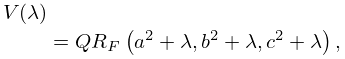
… ►Application of (19.16.23) transforms the last quantity in (19.30.5) into a two-dimensional analog of (19.33.1). … ►

19.33.5

V(\lambda)=QR_{F}\left(a^{2}+\lambda,b^{2}+\lambda,c^{2}+\lambda\right),

ⓘ

Symbols:: $R_{F}\left(\NVar{x},\NVar{y},\NVar{z}\right)$ : symmetric elliptic integral of first kind, $Q$ : charge and $V(\lambda)$ : potential
Permalink:: http://dlmf.nist.gov/19.33.E5
Encodings:: pMML, png, TeX
See also:: Annotations for §19.33(ii), §19.33 and Ch.19

… ►

19.33.6

1/C=R_{F}\left(a^{2},b^{2},c^{2}\right).

ⓘ

Symbols:: $R_{F}\left(\NVar{x},\NVar{y},\NVar{z}\right)$ : symmetric elliptic integral of first kind and $C$ : electric capacity
Permalink:: http://dlmf.nist.gov/19.33.E6
Encodings:: pMML, png, TeX
See also:: Annotations for §19.33(ii), §19.33 and Ch.19

… ►Let a homogeneous magnetic ellipsoid with semiaxes

a, b, c

, volume

V=4\pi abc/3

, and susceptibility

\chi

be placed in a previously uniform magnetic field

H

parallel to the principal axis with semiaxis

c

. The external field and the induced magnetization together produce a uniform field inside the ellipsoid with strength

H/(1+L_{c}\chi)

, where

L_{c}

is the demagnetizing factor, given in cgs units by …

15: 10.16 Relations to Other Functions

… ►

{H^{(1)}_{\frac{1}{2}}}\left(z\right)=-i{H^{(1)}_{-\frac{1}{2}}}\left(z\right)% =-i\left(\frac{2}{\pi z}\right)^{\frac{1}{2}}e^{iz},

… ►

10.16.9

J_{\nu}\left(z\right)=\frac{(\tfrac{1}{2}z)^{\nu}}{\Gamma\left(\nu+1\right)}{{% }_{0}F_{1}}\left(-;\nu+1;-\tfrac{1}{4}z^{2}\right).

ⓘ

Symbols:: $J_{\NVar{\nu}}\left(\NVar{z}\right)$ : Bessel function of the first kind, $\Gamma\left(\NVar{z}\right)$ : gamma function, ${{}_{\NVar{p}}F_{\NVar{q}}}\left(\NVar{a_{1},\dots,a_{p}};\NVar{b_{1},\dots,b_% {q}};\NVar{z}\right)$ or ${{}_{\NVar{p}}F_{\NVar{q}}}\left({\NVar{a_{1},\dots,a_{p}}\atop\NVar{b_{1},% \dots,b_{q}}};\NVar{z}\right)$ : alternatively ${{}_{\NVar{p}}F_{\NVar{q}}}\left(\NVar{\mathbf{a}};\NVar{\mathbf{b}};\NVar{z}\right)$ or ${{}_{\NVar{p}}F_{\NVar{q}}}\left({\NVar{\mathbf{a}}\atop\NVar{\mathbf{b}}};% \NVar{z}\right)$
generalized hypergeometric function, $z$ : complex variable and $\nu$ : complex parameter
Referenced by:: §10.16
Permalink:: http://dlmf.nist.gov/10.16.E9
Encodings:: pMML, png, TeX
See also:: Annotations for §10.16, §10.16 and Ch.10

►For

{{}_{0}F_{1}}

see (16.2.1). ►With

\mathbf{F}

as in §15.2(i), and with

z

and

\nu

fixed, ►

10.16.10

J_{\nu}\left(z\right)=(\tfrac{1}{2}z)^{\nu}\lim\mathbf{F}\left(\lambda,\mu;\nu% +1;-z^{2}/(4\lambda\mu)\right),

ⓘ

Symbols:: $J_{\NVar{\nu}}\left(\NVar{z}\right)$ : Bessel function of the first kind, $\mathbf{F}\left(\NVar{a},\NVar{b};\NVar{c};\NVar{z}\right)$ or $\mathbf{F}\left({\NVar{a},\NVar{b}\atop\NVar{c}};\NVar{z}\right)$ : $={{}_{2}{\mathbf{F}}_{1}}\left(\NVar{a},\NVar{b};\NVar{c};\NVar{z}\right)$ Olver’s hypergeometric function, $z$ : complex variable and $\nu$ : complex parameter
A&S Ref:: 9.1.70 (modified)
Referenced by:: §10.39
Permalink:: http://dlmf.nist.gov/10.16.E10
Encodings:: pMML, png, TeX
See also:: Annotations for §10.16, §10.16 and Ch.10

…

16: 16.11 Asymptotic Expansions

… ►For subsequent use we define two formal infinite series,

E_{p,q}(z)

and

H_{p,q}(z)

, as follows: … ►It may be observed that

H_{p,q}(z)

represents the sum of the residues of the poles of the integrand in (16.5.1) at

s=-a_{j},-a_{j}-1,\dots

j=1,\dots,p

, provided that these poles are all simple, that is, no two of the

a_{j}

differ by an integer. (If this condition is violated, then the definition of

H_{p,q}(z)

has to be modified so that the residues are those associated with the multiple poles. … ►The formal series (16.11.2) for

H_{q+1,q}(z)

converges if

\left|z\right|>1

, and … ►Asymptotic expansions for the polynomials

{{}_{p+2}F_{q}}\left(-r,r+a_{0},\mathbf{a};\mathbf{b};z\right)

r\to\infty

through integer values are given in Fields and Luke (1963b, a) and Fields (1965).

17: 31.2 Differential Equations

… ►

$F$ -Homotopic Transformations

… ►By composing these three steps, there result

2^{3}=8

possible transformations of the dependent variable (including the identity transformation) that preserve the form of (31.2.1). ►

Homographic Transformations

… ►

Composite Transformations

►There are

8\cdot 24=192

automorphisms of equation (31.2.1) by compositions of

F

-homotopic and homographic transformations. …

18: 18.17 Integrals

… ►

§18.17(v) Fourier Transforms

… ►For the beta function

\mathrm{B}\left(a,b\right)

see §5.12, and for the confluent hypergeometric function

{{}_{1}F_{1}}

see (16.2.1) and Chapter 13. … ►For the confluent hypergeometric function

{{}_{1}F_{1}}

see (16.2.1) and Chapter 13. … ►For the hypergeometric function

{{}_{2}F_{1}}

see §§15.1 and 15.2(i). … ►For the generalized hypergeometric function

{{}_{2}F_{2}}

see (16.2.1). …

19: 18.38 Mathematical Applications

… ►with

H_{n}\left(x\right)

as in §18.3, satisfies the Toda equation … ►For the generalized hypergeometric function

{{}_{3}F_{2}}

see (16.2.1). … ►

Radon Transform

… ►The

3j

symbol (34.2.6), with an alternative expression as a terminating

{{}_{3}F_{2}}

of unit argument, can be expressed in terms of Hahn polynomials (18.20.5) or, by (18.21.1), dual Hahn polynomials. … ►The

6j

symbol (34.4.3), with an alternative expression as a terminating balanced

{{}_{4}F_{3}}

of unit argument, can be expressend in terms of Racah polynomials (18.26.3). …

20: 15.9 Relations to Other Functions

… ►

15.9.7

P_{n}\left(x\right)=F\left({-n,n+1\atop 1};\frac{1-x}{2}\right).

ⓘ

Symbols:: $F\left(\NVar{a},\NVar{b};\NVar{c};\NVar{z}\right)$ or $F\left({\NVar{a},\NVar{b}\atop\NVar{c}};\NVar{z}\right)$ : $={{}_{2}F_{1}}\left(\NVar{a},\NVar{b};\NVar{c};\NVar{z}\right)$ Gauss’ hypergeometric function, $P_{\NVar{n}}\left(\NVar{x}\right)$ : Legendre polynomial, $x$ : real variable and $n$ : integer
Permalink:: http://dlmf.nist.gov/15.9.E7
Encodings:: pMML, png, TeX
See also:: Annotations for §15.9(i), §15.9(i), §15.9 and Ch.15

… ►The Jacobi transform is defined as …with inverse … … ►Any hypergeometric function for which a quadratic transformation exists can be expressed in terms of associated Legendre functions or Ferrers functions. …