Euler transformation

SearchAdvancedHelp

(0.004 seconds)

31—40 of 93 matching pages

31: 32.7 Bäcklund Transformations

… ►transforms ${\text{P}}_{\text{VI}}$ with $\alpha =-\beta$ and $\gamma =\frac{1}{2}-\delta$ to ${\text{P}}_{\text{VI}}$ with $({\alpha }_1,{\beta }_1,{\gamma }_1,{\delta }_1)=(4\alpha ,-4\gamma ,0,\frac{1}{2})$. …transforms ${\text{P}}_{\text{VI}}$ with $\alpha =-\beta =\gamma =\frac{1}{2}-\delta$ to ${\text{P}}_{\text{VI}}$ with $({\alpha }_2,{\beta }_2,{\gamma }_2,{\delta }_2)=(16\alpha ,0,0,\frac{1}{2})$. …transforms ${\text{P}}_{\text{VI}}$ with $\alpha =\beta =0$ and $\gamma =\frac{1}{2}-\delta$ to ${\text{P}}_{\text{VI}}$ with ${\alpha }_3={\beta }_3$ and ${\gamma }_3=\frac{1}{2}-{\delta }_3$. …

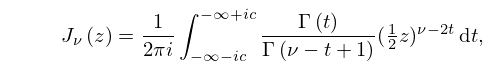
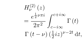
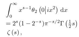
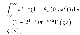
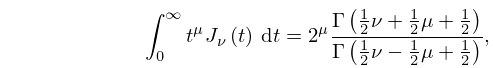
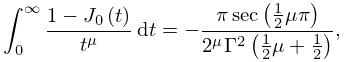
32: 10.9 Integral Representations

… ►

10.9.22 $$J_{\nu }\left(x\right)=\frac{1}{2\pi \mathrm{i}}{\int }_{-\mathrm{i}\mathrm{\infty }}^{\mathrm{i}\mathrm{\infty }}\frac{\mathrm{\Gamma }\left(-t\right){(\frac{1}{2}x)}^{\nu +2t}}{\mathrm{\Gamma }\left(\nu +t+1\right)}dt,$$ $\mathrm{\Re }\nu >0$, $x>0$,

ⓘ

Symbols:

$J_{\nu }\left(z\right)$: Bessel function of the first kind, $\mathrm{\Gamma }\left(z\right)$: gamma function, $\pi$: the ratio of the circumference of a circle to its diameter, $dx$: differential of $x$ , $\mathrm{i}$: imaginary unit, $\int$: integral, $\mathrm{\Re }$: real part, $x$: real variable and $\nu$: complex parameter

Keywords:

Mellin transform

A&S Ref:

9.1.26

Referenced by:

§10.9(ii)

Permalink:

http://dlmf.nist.gov/10.9.E22

Encodings:

pMML, png, TeX

See also:

Annotations for §10.9(ii), §10.9(ii), §10.9 and Ch.10

… ►

10.9.23 $$J_{\nu }\left(z\right)=\frac{1}{2\pi \mathrm{i}}{\int }_{-\mathrm{\infty }-\mathrm{i}c}^{-\mathrm{\infty }+\mathrm{i}c}\frac{\mathrm{\Gamma }\left(t\right)}{\mathrm{\Gamma }\left(\nu -t+1\right)}{(\frac{1}{2}z)}^{\nu -2t}dt,$$

ⓘ

Symbols:

$J_{\nu }\left(z\right)$: Bessel function of the first kind, $\mathrm{\Gamma }\left(z\right)$: gamma function, $\pi$: the ratio of the circumference of a circle to its diameter, $dx$: differential of $x$ , $\mathrm{i}$: imaginary unit, $\int$: integral, $z$: complex variable, $\nu$: complex parameter and $c$: constant

Keywords:

Mellin transform

Permalink:

http://dlmf.nist.gov/10.9.E23

Encodings:

pMML, png, TeX

See also:

Annotations for §10.9(ii), §10.9(ii), §10.9 and Ch.10

… ►

10.9.24 $$H_{\nu }^{(1)}\left(z\right)=-\frac{{\mathrm{e}}^{-\frac{1}{2}\nu \pi \mathrm{i}}}{2{\pi }^2}{\int }_{c-\mathrm{i}\mathrm{\infty }}^{c+\mathrm{i}\mathrm{\infty }}\mathrm{\Gamma }\left(t\right)\mathrm{\Gamma }\left(t-\nu \right){(-\frac{1}{2}\mathrm{i}z)}^{\nu -2t}dt,$$ ,

ⓘ

Symbols:

$\mathrm{\Gamma }\left(z\right)$: gamma function, $H_{\nu }^{(1)}\left(z\right)$: Bessel function of the third kind (or Hankel function), $\pi$: the ratio of the circumference of a circle to its diameter, $dx$: differential of $x$ , $\mathrm{e}$: base of natural logarithm, $\mathrm{i}$: imaginary unit, $\int$: integral, $\mathrm{ph}$: phase, $z$: complex variable, $\nu$: complex parameter and $c$: constant

Keywords:

Mellin transform

Referenced by:

§10.9(ii)

Permalink:

http://dlmf.nist.gov/10.9.E24

Encodings:

pMML, png, TeX

See also:

Annotations for §10.9(ii), §10.9(ii), §10.9 and Ch.10

►

10.9.25 $$H_{\nu }^{(2)}\left(z\right)=\frac{{\mathrm{e}}^{\frac{1}{2}\nu \pi \mathrm{i}}}{2{\pi }^2}{\int }_{c-\mathrm{i}\mathrm{\infty }}^{c+\mathrm{i}\mathrm{\infty }}\mathrm{\Gamma }\left(t\right)\mathrm{\Gamma }\left(t-\nu \right){(\frac{1}{2}\mathrm{i}z)}^{\nu -2t}dt,$$ .

ⓘ

Symbols:

$\mathrm{\Gamma }\left(z\right)$: gamma function, $H_{\nu }^{(2)}\left(z\right)$: Bessel function of the third kind (or Hankel function), $\pi$: the ratio of the circumference of a circle to its diameter, $dx$: differential of $x$ , $\mathrm{e}$: base of natural logarithm, $\mathrm{i}$: imaginary unit, $\int$: integral, $\mathrm{ph}$: phase, $z$: complex variable, $\nu$: complex parameter and $c$: constant

Keywords:

Mellin transform

Referenced by:

§10.9(ii), §10.9(ii)

Permalink:

http://dlmf.nist.gov/10.9.E25

Encodings:

pMML, png, TeX

See also:

Annotations for §10.9(ii), §10.9(ii), §10.9 and Ch.10

… ►

10.9.29 $$J_{\mu }\left(x\right)J_{\nu }\left(x\right)=\frac{1}{2\pi \mathrm{i}}{\int }_{-\mathrm{i}\mathrm{\infty }}^{\mathrm{i}\mathrm{\infty }}\frac{\mathrm{\Gamma }\left(-t\right)\mathrm{\Gamma }\left(2t+\mu +\nu +1\right){(\frac{1}{2}x)}^{\mu +\nu +2t}}{\mathrm{\Gamma }\left(t+\mu +1\right)\mathrm{\Gamma }\left(t+\nu +1\right)\mathrm{\Gamma }\left(t+\mu +\nu +1\right)}dt,$$ $x>0$,

ⓘ

Symbols:

$J_{\nu }\left(z\right)$: Bessel function of the first kind, $\mathrm{\Gamma }\left(z\right)$: gamma function, $\pi$: the ratio of the circumference of a circle to its diameter, $dx$: differential of $x$ , $\mathrm{i}$: imaginary unit, $\int$: integral, $x$: real variable and $\nu$: complex parameter

Keywords:

Mellin transform

Permalink:

http://dlmf.nist.gov/10.9.E29

Encodings:

pMML, png, TeX

See also:

Annotations for §10.9(iii), §10.9(iii), §10.9 and Ch.10

…

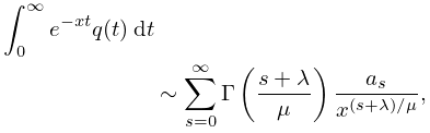
33: 2.3 Integrals of a Real Variable

… ►

2.3.8 $${\int }_0^{\mathrm{\infty }}{\mathrm{e}}^{-xt}q(t)dt\sim \sum _{s=0}^{\mathrm{\infty }}\mathrm{\Gamma }\left(\frac{s+\lambda }{\mu }\right)\frac{a_s}{x^{(s+\lambda )/\mu }},$$ $x\to +\mathrm{\infty }$.

ⓘ

Symbols:

$\mathrm{\Gamma }\left(z\right)$: gamma function, $\sim$: Poincaré asymptotic expansion, $dx$: differential of $x$ , $\mathrm{e}$: base of natural logarithm, $\int$: integral, $a$: positive constant, $q(t)$: function, $\lambda$: positive constant and $\mu$: positive constant

Keywords:

Laplace transform

Referenced by:

§2.3(ii), §2.4(i)

Permalink:

http://dlmf.nist.gov/2.3.E8

Encodings:

pMML, png, TeX

See also:

Annotations for §2.3(ii), §2.3 and Ch.2

…

34: 15.9 Relations to Other Functions

… ►The Jacobi transform is defined as …with inverse ►

15.9.13 $$f(t)=\frac{1}{2\pi \mathrm{i}}{\int }_{-\mathrm{i}\mathrm{\infty }}^{\mathrm{i}\mathrm{\infty }}\tilde{f}(\mathrm{i}\lambda ){\mathrm{\Phi }}_{\mathrm{i}\lambda }^{(\alpha ,\beta )}(t)\frac{\mathrm{\Gamma }\left(\frac{1}{2}(\alpha +\beta +1+\lambda )\right)\mathrm{\Gamma }\left(\frac{1}{2}(\alpha -\beta +1+\lambda )\right)}{\mathrm{\Gamma }\left(\alpha +1\right)\mathrm{\Gamma }\left(\lambda \right)2^{\alpha +\beta +1-\lambda }}d\lambda ,$$

ⓘ

Symbols:

$\mathrm{\Gamma }\left(z\right)$: gamma function, $\pi$: the ratio of the circumference of a circle to its diameter, $dx$: differential of $x$ , $\mathrm{i}$: imaginary unit, $\int$: integral, $(a,b)$: open interval, $f(t)$: function and ${\mathrm{\Phi }}_{\lambda }^{(\alpha ,\beta )}(t)$: function

Permalink:

http://dlmf.nist.gov/15.9.E13

Encodings:

pMML, png, TeX

See also:

Annotations for §15.9(ii), §15.9 and Ch.15

… ► … ►Any hypergeometric function for which a quadratic transformation exists can be expressed in terms of associated Legendre functions or Ferrers functions. …

35: 20.10 Integrals

… ►

20.10.1 $${\int }_0^{\mathrm{\infty }}{x}^{s-1}{\theta }_2\left(0\right|\mathrm{i}{x}^2)dx=2^s(1-2^{-s}){\pi }^{-s/2}\mathrm{\Gamma }\left(\frac{1}{2}s\right)\zeta \left(s\right),$$ $\mathrm{\Re }s>1$,

ⓘ

Symbols:

$\mathrm{\Gamma }\left(z\right)$: gamma function, ${\theta }_j\left(z\right|\tau )$: theta function, $\zeta \left(s\right)$: Riemann zeta function, $\pi$: the ratio of the circumference of a circle to its diameter, $dx$: differential of $x$ , $\mathrm{i}$: imaginary unit, $\int$: integral and $\mathrm{\Re }$: real part

Keywords:

Mellin transform

Referenced by:

§20.10(i), Erratum (V1.1.5) for §20.10(i)

Permalink:

http://dlmf.nist.gov/20.10.E1

Encodings:

pMML, png, TeX

Modification (effective with 1.1.5):

Originally the constraint was $\mathrm{\Re }s>2$. This can be relaxed to $\mathrm{\Re }s>1$ because ${\theta }_2\left(0\right|\mathrm{i}{x}^2)=x^{-1}{\theta }_4\left(0\right|\mathrm{i}{x}^{-2})\sim x^{-1}$ as $x\to 0+$, which follows from (20.7.31) and (20.4.5).

See also:

Annotations for §20.10(i), §20.10 and Ch.20

►

20.10.2 $${\int }_0^{\mathrm{\infty }}{x}^{s-1}({\theta }_3\left(0\right|\mathrm{i}{x}^2)-1)dx={\pi }^{-s/2}\mathrm{\Gamma }\left(\frac{1}{2}s\right)\zeta \left(s\right),$$ $\mathrm{\Re }s>1$,

ⓘ

Symbols:

$\mathrm{\Gamma }\left(z\right)$: gamma function, ${\theta }_j\left(z\right|\tau )$: theta function, $\zeta \left(s\right)$: Riemann zeta function, $\pi$: the ratio of the circumference of a circle to its diameter, $dx$: differential of $x$ , $\mathrm{i}$: imaginary unit, $\int$: integral and $\mathrm{\Re }$: real part

Keywords:

Mellin transform

Referenced by:

§20.10(i), Erratum (V1.1.5) for §20.10(i)

Permalink:

http://dlmf.nist.gov/20.10.E2

Encodings:

pMML, png, TeX

Modification (effective with 1.1.5):

Originally the constraint was $\mathrm{\Re }s>2$. This can be relaxed to $\mathrm{\Re }s>1$ because ${\theta }_3\left(0\right|\mathrm{i}{x}^2)=x^{-1}{\theta }_3\left(0\right|\mathrm{i}{x}^{-2})\sim x^{-1}$ as $x\to 0+$, which follows from (20.7.32) and (20.4.4).

See also:

Annotations for §20.10(i), §20.10 and Ch.20

►

20.10.3 $${\int }_0^{\mathrm{\infty }}{x}^{s-1}(1-{\theta }_4\left(0\right|\mathrm{i}{x}^2))dx=(1-2^{1-s}){\pi }^{-s/2}\mathrm{\Gamma }\left(\frac{1}{2}s\right)\zeta \left(s\right),$$ $\mathrm{\Re }s>0$.

ⓘ

Symbols:

$\mathrm{\Gamma }\left(z\right)$: gamma function, ${\theta }_j\left(z\right|\tau )$: theta function, $\zeta \left(s\right)$: Riemann zeta function, $\pi$: the ratio of the circumference of a circle to its diameter, $dx$: differential of $x$ , $\mathrm{i}$: imaginary unit, $\int$: integral and $\mathrm{\Re }$: real part

Keywords:

Mellin transform

Referenced by:

§20.10(i), Erratum (V1.1.5) for §20.10(i)

Permalink:

http://dlmf.nist.gov/20.10.E3

Encodings:

pMML, png, TeX

Modification (effective with 1.1.5):

Originally the constraint was $\mathrm{\Re }s>2$. This can be relaxed to $\mathrm{\Re }s>0$ because $1-{\theta }_4\left(0\right|\mathrm{i}{x}^2)=1-x^{-1}{\theta }_2\left(0\right|\mathrm{i}{x}^{-2})\sim 1$ as $x\to 0+$, which follows from (20.7.33) and (20.4.3).

See also:

Annotations for §20.10(i), §20.10 and Ch.20

…

36: 15.11 Riemann’s Differential Equation

… ►The importance of (15.10.1) is that any homogeneous linear differential equation of the second order with at most three distinct singularities, all regular, in the extended plane can be transformed into (15.10.1). The most general form is given by … ►Also, if any of $\alpha$, $\beta$, $\gamma$, is at infinity, then we take the corresponding limit in (15.11.1). … ►

§15.11(ii) Transformation Formulas

… ►These constants can be chosen to map any two sets of three distinct points $\{\alpha ,\beta ,\gamma \}$ and $\{\tilde{\alpha },\tilde{\beta },\tilde{\gamma }\}$ onto each other. …

37: 2.4 Contour Integrals

… ►

2.4.4 $$Q(z)\sim \sum _{s=0}^{\mathrm{\infty }}\mathrm{\Gamma }\left(\frac{s+\lambda }{\mu }\right)\frac{a_s}{z^{(s+\lambda )/\mu }},$$ $z\to \mathrm{\infty }$,

ⓘ

Symbols:

$\mathrm{\Gamma }\left(z\right)$: gamma function, $\sim$: Poincaré asymptotic expansion, $\lambda$: constant, $a$: left endpoint, $\mu$: positive constant and $Q(z)$: Laplace transform of $q(t)$

Referenced by:

§2.4(ii)

Permalink:

http://dlmf.nist.gov/2.4.E4

Encodings:

pMML, png, TeX

See also:

Annotations for §2.4(ii), §2.4 and Ch.2

…

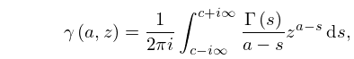
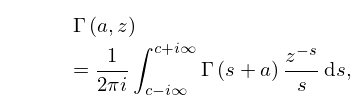
38: 8.6 Integral Representations

… ►

8.6.10 $$\gamma (a,z)=\frac{1}{2\pi \mathrm{i}}{\int }_{c-\mathrm{i}\mathrm{\infty }}^{c+\mathrm{i}\mathrm{\infty }}\frac{\mathrm{\Gamma }\left(s\right)}{a-s}{z}^{a-s}ds,$$ , $a\ne 0,-1,-2,\mathrm{\dots }$,

ⓘ

Symbols:

$\mathrm{\Gamma }\left(z\right)$: gamma function, $\pi$: the ratio of the circumference of a circle to its diameter, $dx$: differential of $x$ , $\mathrm{i}$: imaginary unit, $\gamma (a,z)$: incomplete gamma function, $\int$: integral, $\mathrm{ph}$: phase, $z$: complex variable, $a$: parameter and $c$: real constant

Keywords:

Mellin transform

Referenced by:

§8.6(ii), §8.6(ii), §8.6(ii), Erratum (V1.0.17) for Paragraph Mellin–Barnes Integrals (in §8.6(ii))

Permalink:

http://dlmf.nist.gov/8.6.E10

Encodings:

pMML, png, TeX

See also:

Annotations for §8.6(ii), §8.6(ii), §8.6 and Ch.8

►

8.6.11 $$\mathrm{\Gamma }(a,z)=\frac{1}{2\pi \mathrm{i}}{\int }_{c-\mathrm{i}\mathrm{\infty }}^{c+\mathrm{i}\mathrm{\infty }}\mathrm{\Gamma }\left(s+a\right)\frac{z^{-s}}{s}ds,$$ ,

ⓘ

Symbols:

$\mathrm{\Gamma }\left(z\right)$: gamma function, $\pi$: the ratio of the circumference of a circle to its diameter, $dx$: differential of $x$ , $\mathrm{i}$: imaginary unit, $\mathrm{\Gamma }(a,z)$: incomplete gamma function, $\int$: integral, $\mathrm{ph}$: phase, $z$: complex variable, $a$: parameter and $c$: real constant

Keywords:

Mellin transform

Referenced by:

§8.19(i), §8.6(ii), §8.6(ii), Erratum (V1.0.17) for Paragraph Mellin–Barnes Integrals (in §8.6(ii))

Permalink:

http://dlmf.nist.gov/8.6.E11

Encodings:

pMML, png, TeX

See also:

Annotations for §8.6(ii), §8.6(ii), §8.6 and Ch.8

►

8.6.12 $$\mathrm{\Gamma }(a,z)=-\frac{z^{a-1}{\mathrm{e}}^{-z}}{\mathrm{\Gamma }\left(1-a\right)}\frac{1}{2\pi \mathrm{i}}{\int }_{c-\mathrm{i}\mathrm{\infty }}^{c+\mathrm{i}\mathrm{\infty }}\mathrm{\Gamma }\left(s+1-a\right)\frac{\pi z^{-s}}{\sin \left(\pi s\right)}ds,$$ , $a\ne 1,2,3,\mathrm{\dots }$.

ⓘ

Symbols:

$\mathrm{\Gamma }\left(z\right)$: gamma function, $\pi$: the ratio of the circumference of a circle to its diameter, $dx$: differential of $x$ , $\mathrm{e}$: base of natural logarithm, $\mathrm{i}$: imaginary unit, $\mathrm{\Gamma }(a,z)$: incomplete gamma function, $\int$: integral, $\mathrm{ph}$: phase, $\sin z$: sine function, $z$: complex variable, $a$: parameter and $c$: real constant

Keywords:

Mellin transform

Referenced by:

§8.19(i), §8.6(ii), §8.6(ii), §8.6(ii), Erratum (V1.0.17) for Paragraph Mellin–Barnes Integrals (in §8.6(ii))

Permalink:

http://dlmf.nist.gov/8.6.E12

Encodings:

pMML, png, TeX

See also:

Annotations for §8.6(ii), §8.6(ii), §8.6 and Ch.8

…

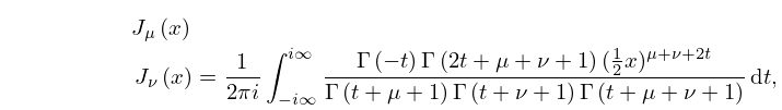
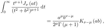
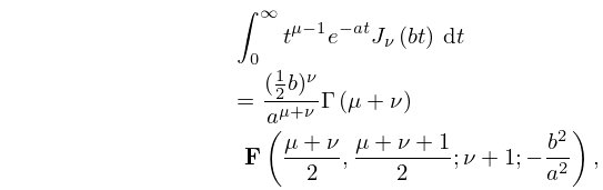
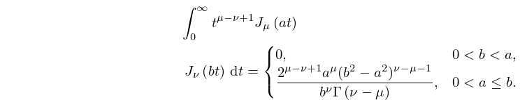
39: 10.22 Integrals

… ►

10.22.43 $${\int }_0^{\mathrm{\infty }}{t}^{\mu }{J}_{\nu }\left(t\right)dt=2^{\mu }\frac{\mathrm{\Gamma }\left(\frac{1}{2}\nu +\frac{1}{2}\mu +\frac{1}{2}\right)}{\mathrm{\Gamma }\left(\frac{1}{2}\nu -\frac{1}{2}\mu +\frac{1}{2}\right)},$$ $\mathrm{\Re }\left(\mu +\nu \right)>-1$, ,

ⓘ

Symbols:

$J_{\nu }\left(z\right)$: Bessel function of the first kind, $\mathrm{\Gamma }\left(z\right)$: gamma function, $dx$: differential of $x$ , $\int$: integral, $\mathrm{\Re }$: real part and $\nu$: complex parameter

Keywords:

Mellin transform

A&S Ref:

11.4.16

Referenced by:

§10.22(iii), §10.59

Permalink:

http://dlmf.nist.gov/10.22.E43

Encodings:

pMML, png, TeX

See also:

Annotations for §10.22(iv), §10.22 and Ch.10

… ►

10.22.45 $${\int }_0^{\mathrm{\infty }}\frac{1-J_0\left(t\right)}{t^{\mu }}dt=-\frac{\pi \sec \left(\frac{1}{2}\mu \pi \right)}{2^{\mu }{\mathrm{\Gamma }}^2\left(\frac{1}{2}\mu +\frac{1}{2}\right)},$$ .

ⓘ

Symbols:

$J_{\nu }\left(z\right)$: Bessel function of the first kind, $\mathrm{\Gamma }\left(z\right)$: gamma function, $\pi$: the ratio of the circumference of a circle to its diameter, $dx$: differential of $x$ , $\int$: integral, $\mathrm{\Re }$: real part and $\sec z$: secant function

Keywords:

Mellin transform

A&S Ref:

11.4.18 (modified)

Referenced by:

§10.22(iv)

Permalink:

http://dlmf.nist.gov/10.22.E45

Encodings:

pMML, png, TeX

See also:

Annotations for §10.22(iv), §10.22 and Ch.10

►

10.22.46 $${\int }_0^{\mathrm{\infty }}\frac{t^{\nu +1}{J}_{\nu }\left(at\right)}{{(t^2+b^2)}^{\mu +1}}dt=\frac{a^{\mu }{b}^{\nu -\mu }}{2^{\mu }\mathrm{\Gamma }\left(\mu +1\right)}{K}_{\nu -\mu }\left(ab\right),$$ $a>0$, $\mathrm{\Re }b>0$, .

ⓘ

Symbols:

$J_{\nu }\left(z\right)$: Bessel function of the first kind, $\mathrm{\Gamma }\left(z\right)$: gamma function, $dx$: differential of $x$ , $\int$: integral, $K_{\nu }\left(z\right)$: modified Bessel function of the second kind, $\mathrm{\Re }$: real part and $\nu$: complex parameter

Keywords:

Mellin transform

A&S Ref:

11.4.44

Referenced by:

§10.22(iv)

Permalink:

http://dlmf.nist.gov/10.22.E46

Encodings:

pMML, png, TeX

See also:

Annotations for §10.22(iv), §10.22 and Ch.10

… ►

10.22.49 $${\int }_0^{\mathrm{\infty }}{t}^{\mu -1}{\mathrm{e}}^{-at}{J}_{\nu }\left(bt\right)dt=\frac{{(\frac{1}{2}b)}^{\nu }}{a^{\mu +\nu }}\mathrm{\Gamma }\left(\mu +\nu \right)𝐅(\frac{\mu +\nu }{2},\frac{\mu +\nu +1}{2};\nu +1;-\frac{b^2}{a^2}),$$ $\mathrm{\Re }\left(\mu +\nu \right)>0,\mathrm{\Re }\left(a\pm \mathrm{i}b\right)>0$,

ⓘ

Symbols:

$J_{\nu }\left(z\right)$: Bessel function of the first kind, $\mathrm{\Gamma }\left(z\right)$: gamma function, $dx$: differential of $x$ , $\mathrm{e}$: base of natural logarithm, $\mathrm{i}$: imaginary unit, $\int$: integral, $\mathrm{\Re }$: real part, $𝐅(a,b;c;z)$ or $𝐅(\genfrac{}{}{0pt}{}{a,b}{c};z)$: $={}_2{}^{}𝐅_1^{}(a,b;c;z)$ Olver’s hypergeometric function and $\nu$: complex parameter

Keywords:

Laplace transform, Mellin transform

Referenced by:

§10.22(iv)

Permalink:

http://dlmf.nist.gov/10.22.E49

Encodings:

pMML, png, TeX

See also:

Annotations for §10.22(iv), §10.22 and Ch.10

… ►

10.22.62

ⓘ

Symbols:

$J_{\nu }\left(z\right)$: Bessel function of the first kind, $\mathrm{\Gamma }\left(z\right)$: gamma function, $dx$: differential of $x$ , $\int$: integral and $\nu$: complex parameter

Keywords:

Mellin transform

A&S Ref:

11.4.41

Referenced by:

§10.22(iv)

Permalink:

http://dlmf.nist.gov/10.22.E62

Encodings:

pMML, png, TeX

See also:

Annotations for §10.22(iv), §10.22(iv), §10.22 and Ch.10

…

40: 16.16 Transformations of Variables

… ►

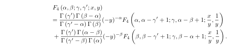
16.16.10 $$F_4(\alpha ,\beta ;\gamma ,{\gamma }^{\prime };x,y)=\frac{\mathrm{\Gamma }\left({\gamma }^{\prime }\right)\mathrm{\Gamma }\left(\beta -\alpha \right)}{\mathrm{\Gamma }\left({\gamma }^{\prime }-\alpha \right)\mathrm{\Gamma }\left(\beta \right)}{(-y)}^{-\alpha }{F}_4(\alpha ,\alpha -{\gamma }^{\prime }+1;\gamma ,\alpha -\beta +1;\frac{x}{y},\frac{1}{y})+\frac{\mathrm{\Gamma }\left({\gamma }^{\prime }\right)\mathrm{\Gamma }\left(\alpha -\beta \right)}{\mathrm{\Gamma }\left({\gamma }^{\prime }-\beta \right)\mathrm{\Gamma }\left(\alpha \right)}{(-y)}^{-\beta }{F}_4(\beta ,\beta -{\gamma }^{\prime }+1;\gamma ,\beta -\alpha +1;\frac{x}{y},\frac{1}{y}).$$

ⓘ

Symbols:

$F_4(\alpha ,\beta ;\gamma ,{\gamma }^{\prime };x,y)$: fourth Appell function and $\mathrm{\Gamma }\left(z\right)$: gamma function

Permalink:

http://dlmf.nist.gov/16.16.E10

Encodings:

pMML, png, TeX

See also:

Annotations for §16.16(ii), §16.16 and Ch.16

…