Euler polynomials
(0.006 seconds)
31—40 of 128 matching pages
31: 18.18 Sums
…
►
18.18.1
…
►
18.18.5
…
►
18.18.14
…
►See Andrews et al. (1999, Lemma 7.1.1) for the more general expansion of in terms of .
…
►
18.18.27
.
…
32: 5.11 Asymptotic Expansions
…
►
5.11.8
…
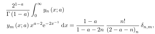
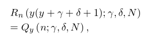
33: 18.34 Bessel Polynomials
…
►
18.34.5_5
.
…
34: 18.25 Wilson Class: Definitions
…
►Table 18.25.1 lists the transformations of variable, orthogonality ranges, and parameter constraints that are needed in §18.2(i) for the Wilson polynomials
, continuous dual Hahn polynomials
, Racah polynomials
, and dual Hahn polynomials
.
►
Table 18.25.1: Wilson class OP’s: transformations of variable, orthogonality ranges, and parameter constraints.
►
►
►
…
►
| OP | Orthogonality range for | Constraints | ||
|---|---|---|---|---|
| … | ||||
| Racah | or or for further constraints see (18.25.1) | |||
| … | ||||
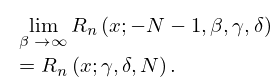
18.25.10
,
…
►
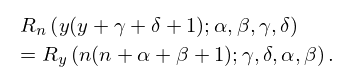
18.25.13
…
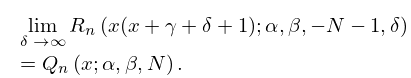
►
18.25.15
…
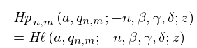
35: 31.5 Solutions Analytic at Three Singularities: Heun Polynomials
…
►
31.5.2
…
36: 18.26 Wilson Class: Continued
37: 3.11 Approximation Techniques
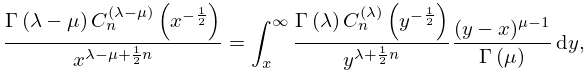
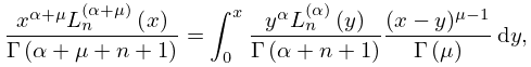
38: 18.17 Integrals
39: 25.6 Integer Arguments
…
►
§25.6(i) Function Values
…40: Errata
…
►
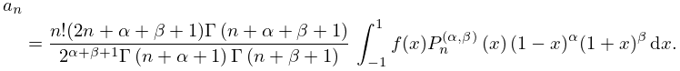
Equation (18.12.2)
…
►
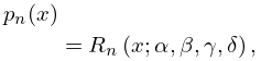
Equation (18.35.5)
…
►
Equation (8.7.6)
…
►
Equations (31.16.2) and (31.16.3)
…
►
Chapter 35 Functions of Matrix Argument
…
18.12.2
This equation was updated to include on the left-hand side, its definition in terms of a product of two functions.
8.7.6
,
The constraint was updated to include “”.
Suggested by Walter Gautschi on 2022-10-14
31.16.2
31.16.3
The generalized hypergeometric function of matrix argument , was linked inadvertently as its single variable counterpart . Furthermore, the Jacobi function of matrix argument , and the Laguerre function of matrix argument , were also linked inadvertently (and incorrectly) in terms of the single variable counterparts given by , and . In order to resolve these inconsistencies, these functions now link correctly to their respective definitions.
