Chebyshev polynomials

(0.006 seconds)

11—20 of 47 matching pages

11: 16.26 Approximations

… ►For discussions of the approximation of generalized hypergeometric functions and the Meijer

G

-function in terms of polynomials, rational functions, and Chebyshev polynomials see Luke (1975, §§5.12 - 5.13) and Luke (1977b, Chapters 1 and 9).

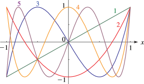
12: 18.4 Graphics

… ►

See accompanying text — Figure 18.4.3: Chebyshev polynomials $T_{n}\left(x\right)$ , $n=1,2,3,4,5$ . Magnify

…

13: 18.13 Continued Fractions

… ►

Chebyshev

►

T_{n}\left(x\right)

is the denominator of the

n

th approximant to: …and

U_{n}\left(x\right)

is the denominator of the

n

th approximant to: …

14: 18.18 Sums

… ►

Chebyshev

►

18.18.21

T_{m}\left(x\right)T_{n}\left(x\right)=\tfrac{1}{2}(T_{m+n}\left(x\right)+T_{m% -n}\left(x\right)).

ⓘ

Symbols:: $T_{\NVar{n}}\left(\NVar{x}\right)$ : Chebyshev polynomial of the first kind, $m$ : nonnegative integer, $n$ : nonnegative integer and $x$ : real variable
Permalink:: http://dlmf.nist.gov/18.18.E21
Encodings:: pMML, png, TeX
See also:: Annotations for §18.18(v), §18.18(v), §18.18 and Ch.18

… ►

18.18.32

2\sum_{\ell=0}^{n}T_{2\ell}\left(x\right)=1+U_{2n}\left(x\right),

ⓘ

Symbols:: $T_{\NVar{n}}\left(\NVar{x}\right)$ : Chebyshev polynomial of the first kind, $U_{\NVar{n}}\left(\NVar{x}\right)$ : Chebyshev polynomial of the second kind, $\ell$ : nonnegative integer, $n$ : nonnegative integer and $x$ : real variable
A&S Ref:: 22.12.2
Referenced by:: §18.18(viii)
Permalink:: http://dlmf.nist.gov/18.18.E32
Encodings:: pMML, png, TeX
See also:: Annotations for §18.18(viii), §18.18(viii), §18.18 and Ch.18

►

18.18.33

2\sum_{\ell=0}^{n}T_{2\ell+1}\left(x\right)=U_{2n+1}\left(x\right),

ⓘ

Symbols:: $T_{\NVar{n}}\left(\NVar{x}\right)$ : Chebyshev polynomial of the first kind, $U_{\NVar{n}}\left(\NVar{x}\right)$ : Chebyshev polynomial of the second kind, $\ell$ : nonnegative integer, $n$ : nonnegative integer and $x$ : real variable
A&S Ref:: 22.12.3
Permalink:: http://dlmf.nist.gov/18.18.E33
Encodings:: pMML, png, TeX
See also:: Annotations for §18.18(viii), §18.18(viii), §18.18 and Ch.18

►

18.18.34

2(1-x^{2})\sum_{\ell=0}^{n}U_{2\ell}\left(x\right)=1-T_{2n+2}\left(x\right),

ⓘ

Symbols:: $T_{\NVar{n}}\left(\NVar{x}\right)$ : Chebyshev polynomial of the first kind, $U_{\NVar{n}}\left(\NVar{x}\right)$ : Chebyshev polynomial of the second kind, $\ell$ : nonnegative integer, $n$ : nonnegative integer and $x$ : real variable
A&S Ref:: 22.12.4
Permalink:: http://dlmf.nist.gov/18.18.E34
Encodings:: pMML, png, TeX
See also:: Annotations for §18.18(viii), §18.18(viii), §18.18 and Ch.18

…

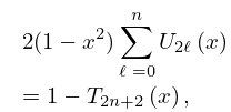
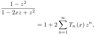
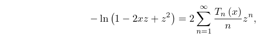
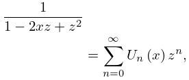
15: 18.12 Generating Functions

… ►

Chebyshev

►

18.12.7

\frac{1-z^{2}}{1-2xz+z^{2}}=1+2\sum_{n=1}^{\infty}T_{n}\left(x\right)z^{n},

|z|<1

ⓘ

Symbols:: $T_{\NVar{n}}\left(\NVar{x}\right)$ : Chebyshev polynomial of the first kind, $z$ : complex variable, $n$ : nonnegative integer and $x$ : real variable
Referenced by:: §18.12
Permalink:: http://dlmf.nist.gov/18.12.E7
Encodings:: pMML, png, TeX
See also:: Annotations for §18.12, §18.12 and Ch.18

►

18.12.8

\frac{1-xz}{1-2xz+z^{2}}=\sum_{n=0}^{\infty}T_{n}\left(x\right)z^{n},

|z|<1

ⓘ

Symbols:: $T_{\NVar{n}}\left(\NVar{x}\right)$ : Chebyshev polynomial of the first kind, $z$ : complex variable, $n$ : nonnegative integer and $x$ : real variable
A&S Ref:: 22.9.6
Referenced by:: §18.12
Permalink:: http://dlmf.nist.gov/18.12.E8
Encodings:: pMML, png, TeX
See also:: Annotations for §18.12, §18.12 and Ch.18

►

18.12.9

-\ln\left(1-2xz+z^{2}\right)=2\sum_{n=1}^{\infty}\frac{T_{n}\left(x\right)}{n}% z^{n},

|z|<1

ⓘ

Symbols:: $T_{\NVar{n}}\left(\NVar{x}\right)$ : Chebyshev polynomial of the first kind, $\ln\NVar{z}$ : principal branch of logarithm function, $z$ : complex variable, $n$ : nonnegative integer and $x$ : real variable
A&S Ref:: 22.9.8
Referenced by:: §18.12
Permalink:: http://dlmf.nist.gov/18.12.E9
Encodings:: pMML, png, TeX
See also:: Annotations for §18.12, §18.12 and Ch.18

►

18.12.10

\frac{1}{1-2xz+z^{2}}=\sum_{n=0}^{\infty}U_{n}\left(x\right)z^{n},

|z|<1

ⓘ

Symbols:: $U_{\NVar{n}}\left(\NVar{x}\right)$ : Chebyshev polynomial of the second kind, $z$ : complex variable, $n$ : nonnegative integer and $x$ : real variable
A&S Ref:: 22.9.10
Referenced by:: §18.12
Permalink:: http://dlmf.nist.gov/18.12.E10
Encodings:: pMML, png, TeX
See also:: Annotations for §18.12, §18.12 and Ch.18

…

16: 3.5 Quadrature

… ►For the latter

a=-1

b=1

, and the nodes

x_{k}

are the extrema of the Chebyshev polynomial

T_{n}\left(x\right)

(§3.11(ii) and §18.3). … ►

Table 3.5.17_5: Recurrence coefficients in (3.5.30) and (3.5.30_5) for monic versions

p_{n}(x)

and orthonormal versions

q_{n}(x)

of the classical orthogonal polynomials.

► ►►►►►►

$p_{n}(x)$	$q_{n}(x)$	$\alpha_{n}$	$\beta_{n}$	$h_{0}$
…
$\frac{1}{k_{n}}T_{n}\left(x\right)$	$\frac{1}{\sqrt{h_{n}}}T_{n}\left(x\right)$	$0$	$\frac{1}{4}\left(1+\delta_{n,1}\right)$	$\pi$
$\frac{1}{k_{n}}U_{n}\left(x\right)$	$\frac{1}{\sqrt{h_{n}}}U_{n}\left(x\right)$	$0$	$\frac{1}{4}$	$\frac{1}{2}\pi$
$\frac{1}{k_{n}}V_{n}\left(x\right)$	$\frac{1}{\sqrt{h_{n}}}V_{n}\left(x\right)$	$\frac{1}{2}\delta_{n,0}$	$\frac{1}{4}$	$\pi$
…
$\frac{1}{k_{n}}T^{*}_{n}\left(x\right)$	$\frac{1}{\sqrt{h_{n}}}T^{*}_{n}\left(x\right)$	$\frac{1}{2}$	$\frac{1}{16}\left(1+\delta_{n,1}\right)$	$\pi$
…

► …

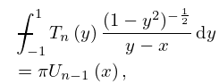
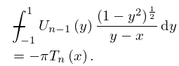
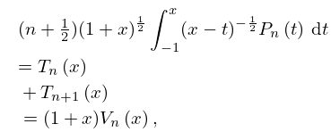
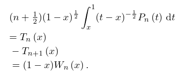
17: 18.17 Integrals

… ►

Chebyshev

►

18.17.42

\pvint_{-1}^{1}T_{n}\left(y\right)\frac{(1-y^{2})^{-\frac{1}{2}}}{y-x}\,% \mathrm{d}y=\pi U_{n-1}\left(x\right),

ⓘ

Symbols:: $T_{\NVar{n}}\left(\NVar{x}\right)$ : Chebyshev polynomial of the first kind, $U_{\NVar{n}}\left(\NVar{x}\right)$ : Chebyshev polynomial of the second kind, $\pi$ : the ratio of the circumference of a circle to its diameter, $\,\mathrm{d}\NVar{x}$ : differential of $x$ , $\pvint_{\NVar{a}}^{\NVar{b}}$ : Cauchy principal value, $y$ : real variable, $n$ : nonnegative integer and $x$ : real variable
A&S Ref:: 22.13.3
Referenced by:: §18.17(viii)
Permalink:: http://dlmf.nist.gov/18.17.E42
Encodings:: pMML, png, TeX
See also:: Annotations for §18.17(viii), §18.17(viii), §18.17 and Ch.18

►

18.17.43

\pvint_{-1}^{1}U_{n-1}\left(y\right)\frac{(1-y^{2})^{\frac{1}{2}}}{y-x}\,% \mathrm{d}y=-\pi T_{n}\left(x\right).

ⓘ

Symbols:: $T_{\NVar{n}}\left(\NVar{x}\right)$ : Chebyshev polynomial of the first kind, $U_{\NVar{n}}\left(\NVar{x}\right)$ : Chebyshev polynomial of the second kind, $\pi$ : the ratio of the circumference of a circle to its diameter, $\,\mathrm{d}\NVar{x}$ : differential of $x$ , $\pvint_{\NVar{a}}^{\NVar{b}}$ : Cauchy principal value, $y$ : real variable, $n$ : nonnegative integer and $x$ : real variable
A&S Ref:: 22.13.4
Referenced by:: §18.17(viii)
Permalink:: http://dlmf.nist.gov/18.17.E43
Encodings:: pMML, png, TeX
See also:: Annotations for §18.17(viii), §18.17(viii), §18.17 and Ch.18

… ►

18.17.45

(n+\tfrac{1}{2})(1+x)^{\frac{1}{2}}\int_{-1}^{x}(x-t)^{-\frac{1}{2}}P_{n}\left% (t\right)\,\mathrm{d}t=T_{n}\left(x\right)+T_{n+1}\left(x\right)=(1+x)V_{n}% \left(x\right),

ⓘ

Symbols:: $T_{\NVar{n}}\left(\NVar{x}\right)$ : Chebyshev polynomial of the first kind, $V_{\NVar{n}}\left(\NVar{x}\right)$ : Chebyshev polynomial of the third kind, $P_{\NVar{n}}\left(\NVar{x}\right)$ : Legendre polynomial, $\,\mathrm{d}\NVar{x}$ : differential of $x$ , $\int$ : integral, $t$ : real variable, $n$ : nonnegative integer and $x$ : real variable
Referenced by:: §18.17(viii), §18.17(viii), §18.18(v), Erratum (V1.2.0) for Equations (18.17.45), (18.17.46)
Permalink:: http://dlmf.nist.gov/18.17.E45
Encodings:: pMML, png, TeX
See also:: Annotations for §18.17(viii), §18.17(viii), §18.17 and Ch.18

►

18.17.46

(n+\tfrac{1}{2})(1-x)^{\frac{1}{2}}\int_{x}^{1}(t-x)^{-\frac{1}{2}}P_{n}\left(% t\right)\,\mathrm{d}t=T_{n}\left(x\right)-T_{n+1}\left(x\right)=(1-x)W_{n}% \left(x\right).

ⓘ

Symbols:: $T_{\NVar{n}}\left(\NVar{x}\right)$ : Chebyshev polynomial of the first kind, $W_{\NVar{n}}\left(\NVar{x}\right)$ : Chebyshev polynomial of the fourth kind, $P_{\NVar{n}}\left(\NVar{x}\right)$ : Legendre polynomial, $\,\mathrm{d}\NVar{x}$ : differential of $x$ , $\int$ : integral, $t$ : real variable, $n$ : nonnegative integer and $x$ : real variable
Referenced by:: §18.17(viii), Erratum (V1.2.0) for Equations (18.17.45), (18.17.46)
Permalink:: http://dlmf.nist.gov/18.17.E46
Encodings:: pMML, png, TeX
See also:: Annotations for §18.17(viii), §18.17(viii), §18.17 and Ch.18

…

18: 18.10 Integral Representations

… ►

Table 18.10.1: Classical OP’s: contour integral representations (18.10.8).

► ►►►►

$p_{n}(x)$	$g_{0}(x)$	$g_{1}(z,x)$	$g_{2}(z,x)$	$c$
…
$T_{n}\left(x\right)$	$1$	$z^{-1}$	$\dfrac{1-xz}{1-2xz+z^{2}}$	$0$
$U_{n}\left(x\right)$	$1$	$z^{-1}$	$(1-2xz+z^{2})^{-1}$	$0$
…

► …

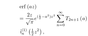
19: 7.6 Series Expansions

… ►

7.6.9

\operatorname{erf}\left(az\right)=\frac{2z}{\sqrt{\pi}}e^{(\frac{1}{2}-a^{2})z% ^{2}}\sum_{n=0}^{\infty}T_{2n+1}\left(a\right){\mathsf{i}^{(1)}_{n}}\left(% \tfrac{1}{2}z^{2}\right),

-1\leq a\leq 1

ⓘ

Symbols:: $T_{\NVar{n}}\left(\NVar{x}\right)$ : Chebyshev polynomial of the first kind, $\pi$ : the ratio of the circumference of a circle to its diameter, $\operatorname{erf}\NVar{z}$ : error function, $\mathrm{e}$ : base of natural logarithm, ${\mathsf{i}^{(1)}_{\NVar{n}}}\left(\NVar{z}\right)$ : modified spherical Bessel function, $z$ : complex variable and $n$ : nonnegative integer
Referenced by:: §7.6(ii)
Permalink:: http://dlmf.nist.gov/7.6.E9
Encodings:: pMML, png, TeX
See also:: Annotations for §7.6(ii), §7.6 and Ch.7

…

20: 18.38 Mathematical Applications

… ►

§18.38(i) Classical OP’s: Numerical Analysis

►

Approximation Theory

►The monic Chebyshev polynomial

2^{1-n}T_{n}\left(x\right)

n\geq 1

, enjoys the ‘minimax’ property on the interval

[-1,1]

, that is,

|2^{1-n}T_{n}\left(x\right)|

has the least maximum value among all monic polynomials of degree

n

. … ►

Differential Equations: Spectral Methods

►Linear ordinary differential equations can be solved directly in series of Chebyshev polynomials (or other OP’s) by a method originated by Clenshaw (1957). …