Cauchy–Schwarz inequalities for sums and integrals

SearchAdvancedHelp

(0.002 seconds)

11—20 of 196 matching pages

11: 19.17 Graphics

… ►

►►

Figure 19.17.6: Cauchy principal value of $R_J(x,y,1,-0.5)$ for $0\le x\le 1$, $y=0,\mathrm{\hspace{0.17em}0.1},\mathrm{\hspace{0.17em}0.5},\mathrm{\hspace{0.17em}1}$. … Magnify

►

►►

Figure 19.17.7: Cauchy principal value of $R_J(0.5,y,1,p)$ for $y=0,\mathrm{\hspace{0.17em}0.01},\mathrm{\hspace{0.17em}0.05},\mathrm{\hspace{0.17em}0.2},\mathrm{\hspace{0.17em}1}$, . … Magnify

…

12: 19.2 Definitions

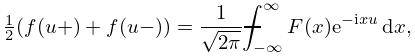
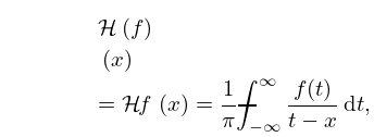
… ►The integral for $E(\varphi ,k)$ is well defined if $k^2={\sin }^2\varphi =1$, and the Cauchy principal value (§1.4(v)) of $\mathrm{\Pi }(\varphi ,{\alpha }^2,k)$ is taken if $1-{\alpha }^2{\sin }^2\varphi$ vanishes at an interior point of the integration path. … ►If , then the integral in (19.2.11) is a Cauchy principal value. … ►Formulas involving $\mathrm{\Pi }(\varphi ,{\alpha }^2,k)$ that are customarily different for circular cases, ordinary hyperbolic cases, and (hyperbolic) Cauchy principal values, are united in a single formula by using $R_C(x,y)$. …

13: Bibliography H

… ►

Applied and Computational Complex Analysis. Vol. 3: Discrete Fourier Analysis—Cauchy Integrals—Construction of Conformal Maps—Univalent Functions. Pure and Applied Mathematics, Wiley-Interscience [John Wiley & Sons Inc.], New York.

ⓘ

Notes:

Reprinted in 1993.

External Links:

ISBN 0-471-08703-3; 0-471-58986-1, MathReview (A. E. Heins), ZentralBlatt

Referenced by:

§1.14(v), Ch.3.

Encodings:

BibTeX

…

14: 19.3 Graphics

… ►

►►

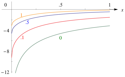
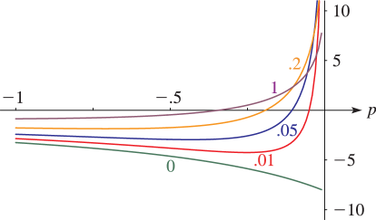
Figure 19.3.2: $R_C(x,1)$ and the Cauchy principal value of $R_C(x,-1)$ for $0\le x\le 5$. … Magnify

… ►

►

►

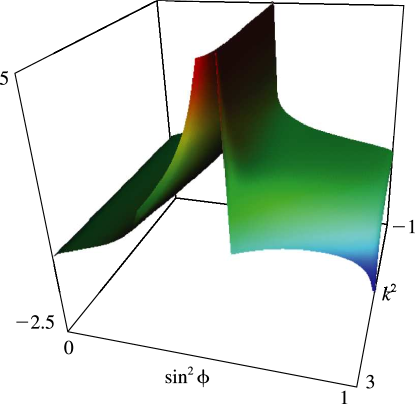
Figure 19.3.6: $\mathrm{\Pi }(\varphi ,2,k)$ as a function of $k^2$ and ${\sin }^2\varphi$ for $-1\le k^2\le 3$, . …If ${\sin }^2\varphi =1$ ($>k^2$), then the function reduces to $\mathrm{\Pi }(2,k)$ with Cauchy principal value $K\left(k\right)-\mathrm{\Pi }(\frac{1}{2}{k}^2,k)$, which tends to $-\mathrm{\infty }$ as $k^2\to 1-$. …If ${\sin }^2\varphi =1/k^2$ (), then by (19.7.4) it reduces to $\mathrm{\Pi }(2/k^2,1/k)/k$, $k^2\ne 2$, with Cauchy principal value $(K\left(1/k\right)-\mathrm{\Pi }(\frac{1}{2},1/k))/k$, , by (19.6.5). … Magnify 3D Help

…

15: 19.22 Quadratic Transformations

… ►

19.22.9 $$\frac{4}{\pi }{R}_G(0,a_0^2,g_0^2)=\frac{1}{M(a_0,g_0)}\left(a_0^2-\sum _{n=0}^{\mathrm{\infty }}{2}^{n-1}{c}_n^2\right)=\frac{1}{M(a_0,g_0)}\left(a_1^2-\sum _{n=2}^{\mathrm{\infty }}{2}^{n-1}{c}_n^2\right),$$

ⓘ

Symbols:

$R_G(x,y,z)$: symmetric elliptic integral of second kind, $M(a,g)$: arithmetic-geometric mean, $\pi$: the ratio of the circumference of a circle to its diameter, $n$: nonnegative integer, $a_n$: iterate and $g_n$: iterate

Permalink:

http://dlmf.nist.gov/19.22.E9

Encodings:

pMML, png, TeX

See also:

Annotations for §19.22(ii), §19.22 and Ch.19

… ►

19.22.10 $$R_D(0,g_0^2,a_0^2)=\frac{3\pi }{4M(a_0,g_0)a_0^2}\sum _{n=0}^{\mathrm{\infty }}{Q}_n,$$

ⓘ

Symbols:

$R_D(x,y,z)$: elliptic integral symmetric in only two variables, $M(a,g)$: arithmetic-geometric mean, $\pi$: the ratio of the circumference of a circle to its diameter, $n$: nonnegative integer, $Q_n$ , $a_n$: iterate and $g_n$: iterate

Referenced by:

§19.22(ii)

Permalink:

http://dlmf.nist.gov/19.22.E10

Encodings:

pMML, png, TeX

See also:

Annotations for §19.22(ii), §19.22 and Ch.19

… ►

19.22.12 $$R_J(0,g_0^2,a_0^2,p_0^2)=\frac{3\pi }{4M(a_0,g_0)p_0^2}\sum _{n=0}^{\mathrm{\infty }}{Q}_n,$$

ⓘ

Symbols:

$R_J(x,y,z,p)$: symmetric elliptic integral of third kind, $M(a,g)$: arithmetic-geometric mean, $\pi$: the ratio of the circumference of a circle to its diameter, $n$: nonnegative integer, $Q_n$ , $p_j$: coefficient, $a_n$: iterate and $g_n$: iterate

Referenced by:

§19.8(i)

Permalink:

http://dlmf.nist.gov/19.22.E12

Encodings:

pMML, png, TeX

See also:

Annotations for §19.22(ii), §19.22 and Ch.19

… ►If the last variable of $R_J$ is negative, then the Cauchy principal value is ►

19.22.14 $$R_J(0,g_0^2,a_0^2,-q_0^2)=\frac{-3\pi }{4M(a_0,g_0)(q_0^2+a_0^2)}\left(2+\frac{a_0^2-g_0^2}{q_0^2+g_0^2}\sum _{n=0}^{\mathrm{\infty }}{Q}_n\right),$$

ⓘ

Symbols:

$R_J(x,y,z,p)$: symmetric elliptic integral of third kind, $M(a,g)$: arithmetic-geometric mean, $\pi$: the ratio of the circumference of a circle to its diameter, $n$: nonnegative integer, $Q_n$ , $a_n$: iterate and $g_n$: iterate

Permalink:

http://dlmf.nist.gov/19.22.E14

Encodings:

pMML, png, TeX

See also:

Annotations for §19.22(ii), §19.22 and Ch.19

…

16: 1.10 Functions of a Complex Variable

… ►

1.10.8 $$\frac{1}{2\pi \mathrm{i}}{\int }_{C}f(z)dz=\text{<span class="ltx\_text hilite">sum</span> of the residues of }f(z)\text{ within }C.$$

ⓘ

Symbols:

$\pi$: the ratio of the circumference of a circle to its diameter, $dx$: differential of $x$ , $\mathrm{i}$: imaginary unit, $\int$: integral, $z$: variable and $C$: closed contour

Referenced by:

§2.10(iii)

Permalink:

http://dlmf.nist.gov/1.10.E8

Encodings:

pMML, png, TeX

See also:

Annotations for §1.10(iv), §1.10 and Ch.1

… ►

1.10.10 $$\frac{1}{2\pi \mathrm{i}}{\int }_C\frac{z{f}^{\prime }(z)}{f(z)}dz=\text{(<span class="ltx\_text hilite">sum</span> of locations of zeros)}-\text{(<span class="ltx\_text hilite">sum</span> of locations of poles)},$$

ⓘ

Symbols:

$\pi$: the ratio of the circumference of a circle to its diameter, $dx$: differential of $x$ , $\mathrm{i}$: imaginary unit, $\int$: integral, $z$: variable and $C$: closed contour

Permalink:

http://dlmf.nist.gov/1.10.E10

Encodings:

pMML, png, TeX

See also:

Annotations for §1.10(iv), §1.10(iv), §1.10 and Ch.1

…

17: 19.36 Methods of Computation

… ►All cases of $R_F$, $R_C$, $R_J$, and $R_D$ are computed by essentially the same procedure (after transforming Cauchy principal values by means of (19.20.14) and (19.2.20)). … ►

19.36.13 $$2R_G(t_0^2,t_0^2+\theta c_0^2,t_0^2+\theta a_0^2)=\left(t_0^2+\theta \sum _{m=0}^{\mathrm{\infty }}{2}^{m-1}{c}_m^2\right)R_C(T^2+\theta M^2,T^2)+h_0+\sum _{m=1}^{\mathrm{\infty }}{2}^m(h_m-h_{m-1}).$$

ⓘ

Symbols:

$R_C(x,y)$: Carlson’s combination of inverse circular and inverse hyperbolic functions, $R_G(x,y,z)$: symmetric elliptic integral of second kind, $m$: nonnegative integer, $M$: limit, $T$: limit and $h_n$

Permalink:

http://dlmf.nist.gov/19.36.E13

Encodings:

pMML, png, TeX

See also:

Annotations for §19.36(ii), §19.36(ii), §19.36 and Ch.19

…

18: 1.14 Integral Transforms

… ►

1.14.3 $$\frac{1}{2}(f(u+)+f(u-))=\frac{1}{\sqrt{2\pi }}{⨍}_{-\mathrm{\infty }}^{\mathrm{\infty }}F(x){\mathrm{e}}^{-\mathrm{i}xu}dx,$$

ⓘ

Symbols:

$\pi$: the ratio of the circumference of a circle to its diameter, $dx$: differential of $x$ , $\mathrm{e}$: base of natural logarithm, $\mathrm{i}$: imaginary unit, ${⨍}_a^b$: Cauchy principal value and $F(x)$: Fourier transform of $f(t)$

Permalink:

http://dlmf.nist.gov/1.14.E3

Encodings:

pMML, png, TeX

See also:

Annotations for §1.14(i), §1.14(i), §1.14 and Ch.1

►where the last integral denotes the Cauchy principal value (1.4.25). … ►

1.14.41 $$\mathscr{H}\left(f\right)\left(x\right)=\mathscr{H}f\left(x\right)=\frac{1}{\pi }{⨍}_{-\mathrm{\infty }}^{\mathrm{\infty }}\frac{f(t)}{t-x}dt,$$

ⓘ

Symbols:

$\mathscr{H}\left(f\right)\left(x\right)$: Hilbert transform, $\pi$: the ratio of the circumference of a circle to its diameter, $dx$: differential of $x$ and ${⨍}_a^b$: Cauchy principal value

Permalink:

http://dlmf.nist.gov/1.14.E41

Encodings:

pMML, png, TeX

Notational Change (effective with 1.0.15):

The notation for the Hilbert transform was changed to $\mathscr{H}\left(f\right)\left(x\right)$ or $\mathscr{H}f\left(x\right)$ from $\mathscr{H}(f;x)$.

See also:

Annotations for §1.14(v), §1.14 and Ch.1

… ►

1.14.44 $$f(x)=-\frac{1}{\pi }{⨍}_{-\mathrm{\infty }}^{\mathrm{\infty }}\frac{\mathscr{H}f\left(u\right)}{u-x}du.$$

ⓘ

Symbols:

$\mathscr{H}\left(f\right)\left(x\right)$: Hilbert transform, $\pi$: the ratio of the circumference of a circle to its diameter, $dx$: differential of $x$ and ${⨍}_a^b$: Cauchy principal value

Referenced by:

§1.14(v)

Permalink:

http://dlmf.nist.gov/1.14.E44

Encodings:

pMML, png, TeX

Notational Change (effective with 1.0.15):

The notation for the Hilbert transform was changed to $\mathscr{H}f\left(u\right)$ from $\mathscr{H}(f;u)$.

See also:

Annotations for §1.14(v), §1.14(v), §1.14 and Ch.1

…

19: 19.24 Inequalities

… ►

§19.24(i) Complete Integrals

… ► ►

§19.24(ii) Incomplete Integrals

… ►Inequalities for $R_C(x,y)$ and $R_D(x,y,z)$ are included as special cases (see (19.16.6) and (19.16.5)). ►Other inequalities for $R_F(x,y,z)$ are given in Carlson (1970). …

20: 6.8 Inequalities

§6.8 Inequalities

…