DLMF: Untitled Document

… ►Abramowitz and Stegun (1964, Chapter 23) includes exact values of

\sum_{k=1}^{m}k^{n}

,

m=1(1)100

,

n=1(1)10

;

\sum_{k=1}^{\infty}k^{-n}

,

\sum_{k=1}^{\infty}(-1)^{k-1}k^{-n}

,

\sum_{k=0}^{\infty}(2k+1)^{-n}

,

n=1,2,\dotsc

, 20D;

\sum_{k=0}^{\infty}(-1)^{k}(2k+1)^{-n}

,

n=1,2,\dotsc

, 18D. ►Wagstaff (1978) gives complete prime factorizations of

N_{n}

and

E_{n}

for

n=20(2)60

and

n=8(2)42

, respectively. … ►For information on tables published before 1961 see Fletcher et al. (1962, v. 1, §4) and Lebedev and Fedorova (1960, Chapters 11 and 14).

… ►

D. E. Amos (1983c) Uniform asymptotic expansions for exponential integrals

E_{n}(x)

and Bickley functions

{\rm{K}i}_{n}(x)

. ACM Trans. Math. Software 9 (4), pp. 467–479.

ⓘ

External Links:: ISSN 0098-3500, Document, MathReview (Marietta J. Tretter), ZentralBlatt
Referenced by:: §10.43(iii).
Encodings:: BibTeX

… ►

K. Aomoto (1987) Special value of the hypergeometric function

{}_{3}F_{2}

and connection formulae among asymptotic expansions. J. Indian Math. Soc. (N.S.) 51, pp. 161–221.

ⓘ

External Links:: ISSN 0019-5839, MathReview (R. A. Askey), ZentralBlatt
Referenced by:: §16.4(iii).
Encodings:: BibTeX

… ►

A. Apelblat (1989) Derivatives and integrals with respect to the order of the Struve functions

\mathbf{H}_{\nu}(x)

and

\mathbf{L}_{\nu}(x)

. J. Math. Anal. Appl. 137 (1), pp. 17–36.

ⓘ

External Links:: ISSN 0022-247X, Document, MathReview (A. McD. Mercer), ZentralBlatt
Referenced by:: §11.4(vi), §11.7(iv).
Encodings:: BibTeX

… ►

R. W. B. Ardill and K. J. M. Moriarty (1978) Spherical Bessel functions

j_{n}

and

y_{n}

of integer order and real argument. Comput. Phys. Comm. 14 (3-4), pp. 261–265.

ⓘ

Notes:: Single-precision Fortran, maximum accuracy 10S.
External Links:: ISSN 0010-4655, Document, Code
Referenced by:: 1st item.
Encodings:: BibTeX

… ►

V. I. Arnol’d (1972) Normal forms of functions near degenerate critical points, the Weyl groups

{A}_{k},{D}_{k},{E}_{k}

and Lagrangian singularities. Funkcional. Anal. i Priložen. 6 (4), pp. 3–25 (Russian).

ⓘ

Notes:: In Russian. English translation: Functional Anal. Appl., 6(1973), pp. 254–272.
External Links:: MathReview (G. R. Belickii), ZentralBlatt
Referenced by:: §36.2(i).
Encodings:: BibTeX

…

… ►

M. K. Kerimov and S. L. Skorokhodov (1984c) Evaluation of complex zeros of Bessel functions

J_{\nu}(z)

and

I_{\nu}(z)

and their derivatives. Zh. Vychisl. Mat. i Mat. Fiz. 24 (10), pp. 1497–1513.

ⓘ

Notes:: English translation in U.S.S.R. Computational Math. and Math. Phys. 24(5), pp. 131–141
External Links:: ISSN 0044-4669, Document, MathReview (Walter Gautschi), ZentralBlatt
Referenced by:: §10.21(ix), §10.74(vi), 4th item.
Encodings:: BibTeX

… ►

S. K. Kim (1972) The asymptotic expansion of a hypergeometric function

{}_{2}F_{2}(1,\,\alpha;\,\rho_{1},\,\rho_{2};\,z)

. Math. Comp. 26 (120), pp. 963.

ⓘ

External Links:: FullText, MathReview, ZentralBlatt
Referenced by:: §16.11(ii), §16.11(ii).
Encodings:: BibTeX

… ►

Y. S. Kim, A. K. Rathie, and R. B. Paris (2013) An extension of Saalschütz’s summation theorem for the series

{}_{r+3}F_{r+2}

. Integral Transforms Spec. Funct. 24 (11), pp. 916–921.

ⓘ

External Links:: ISSN 1065-2469, Document, FullText, MathReview (Christian Lavault), ZentralBlatt
Referenced by:: §16.4(ii), §16.4(ii).
Encodings:: BibTeX

… ►

C. G. Kokologiannaki, P. D. Siafarikas, and C. B. Kouris (1992) On the complex zeros of

H_{\mu}(z),\ J^{\prime}_{\mu}(z),\ J^{\prime\prime}_{\mu}(z)

for real or complex order. J. Comput. Appl. Math. 40 (3), pp. 337–344.

ⓘ

External Links:: ISSN 0377-0427, Document, MathReview, ZentralBlatt
Referenced by:: §10.21(ix).
Encodings:: BibTeX

… ►

E. D. Krupnikov and K. S. Kölbig (1997) Some special cases of the generalized hypergeometric function

{}_{q+1}F_{q}

. J. Comput. Appl. Math. 78 (1), pp. 79–95.

ⓘ

External Links:: ISSN 0377-0427, Document, MathReview (Boro Döring), ZentralBlatt
Referenced by:: §16.7.
Encodings:: BibTeX

…

… ►

26.12.9

\left(\prod_{h=1}^{r}\prod_{j=1}^{s}\frac{h+j+t-1}{h+j-1}\right)^{2};

ⓘ

Symbols:: $r$ : positive integer, $s$ : positive integer, $t$ : positive integer, $h$ : positive integer and $j$ : positive integer
Permalink:: http://dlmf.nist.gov/26.12.E9
Encodings:: pMML, png, TeX
See also:: Annotations for §26.12(i), §26.12 and Ch.26

… ►

26.12.10

\left(\prod_{h=1}^{r}\prod_{j=1}^{s}\frac{h+j+t-1}{h+j-1}\right)\*\left(\prod_% {h=1}^{r+1}\prod_{j=1}^{s}\frac{h+j+t-1}{h+j-1}\right);

ⓘ

Symbols:: $r$ : positive integer, $s$ : positive integer, $t$ : positive integer, $h$ : positive integer and $j$ : positive integer
Permalink:: http://dlmf.nist.gov/26.12.E10
Encodings:: pMML, png, TeX
See also:: Annotations for §26.12(i), §26.12 and Ch.26

… ►

26.12.11

\left(\prod_{h=1}^{r+1}\prod_{j=1}^{s}\frac{h+j+t-1}{h+j-1}\right)\*\left(% \prod_{h=1}^{r}\prod_{j=1}^{s+1}\frac{h+j+t-1}{h+j-1}\right).

ⓘ

Symbols:: $r$ : positive integer, $s$ : positive integer, $t$ : positive integer, $h$ : positive integer and $j$ : positive integer
Permalink:: http://dlmf.nist.gov/26.12.E11
Encodings:: pMML, png, TeX
See also:: Annotations for §26.12(i), §26.12 and Ch.26

… ►The notation

\sum_{\pi\subseteq B(r,s,t)}

denotes the sum over all plane partitions contained in

B(r,s,t)

, and

|\pi|

denotes the number of elements in

\pi

. … ►where

\sigma_{2}(j)

is the sum of the squares of the divisors of

j

. …

… ►

•

Wills et al. (1982) tabulates $j_{0,m}$ , $j_{1,m}$ , $y_{0,m}$ , $y_{1,m}$ for $m=1(1)30$ , 35D.

… ►

•

MacDonald (1989) tabulates the first 30 zeros, in ascending order of absolute value in the fourth quadrant, of the function $J_{0}\left(z\right)-iJ_{1}\left(z\right)$ , 6D. (Other zeros of this function can be obtained by reflection in the imaginary axis).

… ►

•

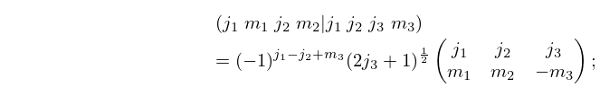
Abramowitz and Stegun (1964, Chapter 11) tabulates $\int_{0}^{x}J_{0}\left(t\right)\,\mathrm{d}t$ , $\int_{0}^{x}Y_{0}\left(t\right)\,\mathrm{d}t$ , $x=0(.1)10$ , 10D; $\int_{0}^{x}t^{-1}(1-J_{0}\left(t\right))\,\mathrm{d}t$ , $\int_{x}^{\infty}t^{-1}Y_{0}\left(t\right)\,\mathrm{d}t$ , $x=0(.1)5$ , 8D.

… ►

•

Abramowitz and Stegun (1964, Chapter 11) tabulates $e^{-x}\int_{0}^{x}I_{0}\left(t\right)\,\mathrm{d}t$ , $e^{x}\int_{x}^{\infty}K_{0}\left(t\right)\,\mathrm{d}t$ , $x=0(.1)10$ , 7D; $e^{-x}\int_{0}^{x}t^{-1}(I_{0}\left(t\right)-1)\,\mathrm{d}t$ , $xe^{x}\int_{x}^{\infty}t^{-1}K_{0}\left(t\right)\,\mathrm{d}t$ , $x=0(.1)5$ , 6D.

… ►

•

Zhang and Jin (1996, pp. 296–305) tabulates $\mathsf{j}_{n}\left(x\right)$ , $\mathsf{j}_{n}'\left(x\right)$ , $\mathsf{y}_{n}\left(x\right)$ , $\mathsf{y}_{n}'\left(x\right)$ , ${\mathsf{i}^{(1)}_{n}}\left(x\right)$ , ${\mathsf{i}^{(1)}_{n}}'\left(x\right)$ , $\mathsf{k}_{n}\left(x\right)$ , $\mathsf{k}_{n}'\left(x\right)$ , $n=0(1)10(10)30$ , 50, 100, $x=1$ , 5, 10, 25, 50, 100, 8S; $x\mathsf{j}_{n}\left(x\right)$ , $(x\mathsf{j}_{n}\left(x\right))^{\prime}$ , $x\mathsf{y}_{n}\left(x\right)$ , $(x\mathsf{y}_{n}\left(x\right))^{\prime}$ (Riccati–Bessel functions and their derivatives), $n=0(1)10(10)30$ , 50, 100, $x=1$ , 5, 10, 25, 50, 100, 8S; real and imaginary parts of $\mathsf{j}_{n}\left(z\right)$ , $\mathsf{j}_{n}'\left(z\right)$ , $\mathsf{y}_{n}\left(z\right)$ , $\mathsf{y}_{n}'\left(z\right)$ , ${\mathsf{i}^{(1)}_{n}}\left(z\right)$ , ${\mathsf{i}^{(1)}_{n}}'\left(z\right)$ , $\mathsf{k}_{n}\left(z\right)$ , $\mathsf{k}_{n}'\left(z\right)$ , $n=0(1)15$ , 20(10)50, 100, $z=4+2i$ , $20+10i$ , 8S. (For the notation replace $j, y, i, k$ by $\mathsf{j}$ , $\mathsf{y}$ , ${\mathsf{i}^{(1)}}$ , $\mathsf{k}$ , respectively.)

…

… ►

\begin{pmatrix}j_{1}&j_{2}&j_{3}\\ m_{1}&m_{2}&m_{3}\end{pmatrix},

►

\begin{Bmatrix}j_{1}&j_{2}&j_{3}\\ l_{1}&l_{2}&l_{3}\end{Bmatrix},

►

\begin{Bmatrix}j_{11}&j_{12}&j_{13}\\ j_{21}&j_{22}&j_{23}\\ j_{31}&j_{32}&j_{33}\end{Bmatrix}.

►An often used alternative to the

\mathit{3j}

symbol is the Clebsch–Gordan coefficient ►

34.1.1

\left(j_{1}\;m_{1}\;j_{2}\;m_{2}|j_{1}\;j_{2}\;j_{3}\,\,m_{3}\right)=(-1)^{j_{% 1}-j_{2}+m_{3}}(2j_{3}+1)^{\frac{1}{2}}\begin{pmatrix}j_{1}&j_{2}&j_{3}\\ m_{1}&m_{2}&-m_{3}\end{pmatrix};

ⓘ

Symbols:: $\begin{pmatrix}\NVar{j_{1}}&\NVar{j_{2}}&\NVar{j_{3}}\\ \NVar{m_{1}}&\NVar{m_{2}}&\NVar{m_{3}}\end{pmatrix}$ : $\mathit{3j}$ symbol and $j,j_{r}$ : non-negative integers or non-negative integers plus one half.
Sources:: Edmonds (1974, p. 46, Eq. (3.7.3)); Rotenberg et al. (1959, p. 1, Eq. (1.1a))
Permalink:: http://dlmf.nist.gov/34.1.E1
Encodings:: pMML, png, TeX
Clarification (effective with 1.0.15):: A wording change reflects that the Clebsch–Gordan coefficients are an alternative formulation of angular momentum problems, rather than alternative notation for the $\mathit{3j}$ . The sign of $m_{3}$ was changed for clarity.
See also:: Annotations for §34.1 and Ch.34

…

… ►The cofactor

A_{jk}

of

a_{jk}

is … ►For real-valued

a_{jk}

, … ►where

\omega_{1},\omega_{2},\dots,\omega_{n}

are the

n

th roots of unity (1.11.21). … ►If

D_{n}[a_{j,k}]

tends to a limit

L

as

n\to\infty

, then we say that the infinite determinant

D_{\infty}[a_{j,k}]

converges and

D_{\infty}[a_{j,k}]=L

. … ►The corresponding eigenvectors

\mathbf{a}_{1},\dots,\mathbf{a}_{n}

can be chosen such that they form a complete orthonormal basis in

\mathbf{E}_{n}

. …

… ►Let

S=\{1^{a_{1}},2^{a_{2}},\ldots,n^{a_{n}}\}

be the multiset that has

a_{j}

copies of

j

,

1\leq j\leq n

.

\mathfrak{S}_{S}

denotes the set of permutations of

S

for all distinct orderings of the

a_{1}+a_{2}+\cdots+a_{n}

integers. The number of elements in

\mathfrak{S}_{S}

is the multinomial coefficient (§26.4)

\genfrac{(}{)}{0.0pt}{}{a_{1}+a_{2}+\cdots+a_{n}}{a_{1},a_{2},\ldots,a_{n}}

. … ►The $q$ -multinomial coefficient is defined in terms of Gaussian polynomials (§26.9(ii)) by …and again with

S=\{1^{a_{1}},2^{a_{2}},\ldots,n^{a_{n}}\}

we have …

… ►

See accompanying text — Figure 30.7.4: Eigenvalues $\lambda^{10}_{n}\left(\gamma^{2}\right)$ , $n=10,11,12,13$ , $-50\leq\gamma^{2}\leq 150$ . Magnify

… ►

►

…

… ►Equations (24.5.3) and (24.5.4) enable

B_{n}

and

E_{n}

to be computed by recurrence. …For example, the tangent numbers

T_{n}

can be generated by simple recurrence relations obtained from (24.15.3), then (24.15.4) is applied. … ►For other information see Chellali (1988) and Zhang and Jin (1996, pp. 1–11). For algorithms for computing

B_{n}

,

E_{n}

,

B_{n}\left(x\right)

, and

E_{n}\left(x\right)

see Spanier and Oldham (1987, pp. 37, 41, 171, and 179–180). ►

§24.19(ii) Values of $B_{n}$ Modulo $p$

…

.足球彩票世界杯玩法__『welcom_』_世界杯用球_w6n2c9o_2022年11月30日22时40分37秒_ttnjbxtnd.com

11—20 of 783 matching pages

11: 24.20 Tables

12: Bibliography

13: Bibliography K

14: 26.12 Plane Partitions

15: 10.75 Tables

16: 34.1 Special Notation

17: 1.3 Determinants, Linear Operators, and Spectral Expansions

18: 26.16 Multiset Permutations

19: 30.7 Graphics

20: 24.19 Methods of Computation

§24.19(ii) Values of $B_{n}$ Modulo $p$

.足球彩票世界杯玩法__『welcom_』_世界杯用球_w6n2c9o_2022年11月30日22时40分37秒_ttnjbxtnd.com

11—20 of 783 matching pages

11: 24.20 Tables

12: Bibliography

13: Bibliography K

14: 26.12 Plane Partitions

15: 10.75 Tables

16: 34.1 Special Notation

17: 1.3 Determinants, Linear Operators, and Spectral Expansions

18: 26.16 Multiset Permutations

19: 30.7 Graphics

20: 24.19 Methods of Computation

§24.19(ii) Values of B n Modulo p

§24.19(ii) Values of $B_{n}$ Modulo $p$