.今年世界杯对阵__『wn4.com_』_巴西世界杯梅西金球奖_w6n2c9o_2022年11月30日8时7分_lvhhtouai.com
(0.012 seconds)
21—30 of 783 matching pages
21: 16.11 Asymptotic Expansions
…
►For subsequent use we define two formal infinite series, and , as follows:
…and .
Explicit representations for the coefficients are given in Volkmer (2023).
…
►In this subsection we assume that none of is a nonpositive integer.
…
►Explicit representations for the coefficients are given in Volkmer and Wood (2014).
…
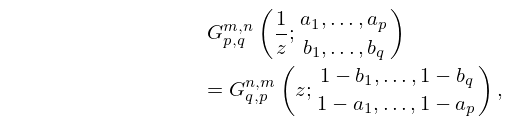
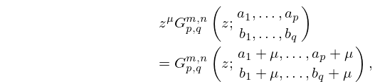
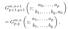
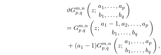
22: 16.19 Identities
23: 1.3 Determinants, Linear Operators, and Spectral Expansions
…
►The cofactor
of is
…
►For real-valued ,
…
►where are the th roots of unity (1.11.21).
…
►If tends to a limit as , then we say that the infinite determinant
converges and .
…
►The corresponding eigenvectors can be chosen such that they form a complete orthonormal basis in .
…
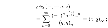
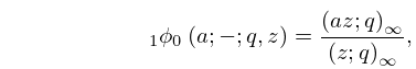
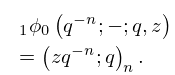
24: 17.5 Functions
25: 16.8 Differential Equations
…
►is a value of at which all the coefficients , , are analytic.
If is not an ordinary point but , , are analytic at , then is a regular singularity.
…
►where and are constants.
…
►where indicates that the entry is omitted.
…
►where indicates that the entry is omitted.
…
26: 3.6 Linear Difference Equations
…
►Given numerical values of and , the solution of the equation
…These errors have the effect of perturbing the solution by unwanted small multiples of and of an independent solution , say.
…
►The unwanted multiples of now decay in comparison with , hence are of little consequence.
…
►The latter method is usually superior when the true value of is zero or pathologically small.
…
►beginning with .
…
27: 16.2 Definition and Analytic Properties
…
►Throughout this chapter it is assumed that none of the bottom parameters , , , is a nonpositive integer, unless stated otherwise. Then formally
…Equivalently, the function is denoted by or , and sometimes, for brevity, by .
…
►Suppose first one or more of the top parameters is a nonpositive integer.
…
►See §16.5 for the definition of as a contour integral when and none of the is a nonpositive integer.
…
►When and is fixed and not a branch point, any branch of is an entire function of each of the parameters .
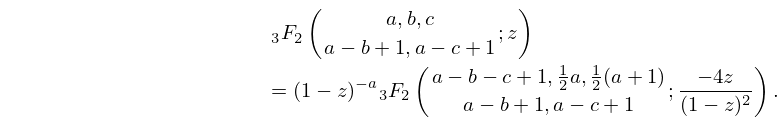
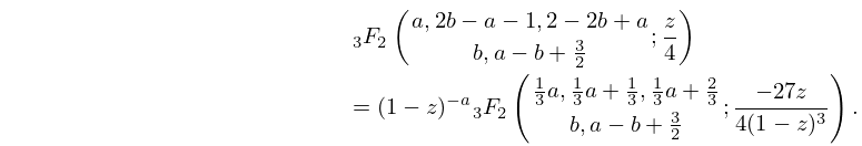
28: 16.6 Transformations of Variable
…
►
16.6.1
…
►
16.6.2
►For Kummer-type transformations of functions see Miller (2003) and Paris (2005a), and for further transformations see Erdélyi et al. (1953a, §4.5), Miller and Paris (2011), Choi and Rathie (2013) and Wang and Rathie (2013).
29: 17.9 Further Transformations of Functions
…
►
