.%E9%A3%9E%E9%B8%9F%E6%8E%92%E9%98%9F%E8%91%A1%E8%90%84%E7%89%99%E7%90%83%E9%98%9F%E7%BD%91%E5%9D%80%E3%80%8E%E4%B8%96%E7%95%8C%E6%9D%AF%E4%BD%A3%E9%87%91%E5%88%86%E7%BA%A255%25%EF%BC%8C%E5%92%A8%E8%AF%A2%E4%B8%93%E5%91%98%EF%BC%9A%40ky975%E3%80%8F.wag.k2q1w9-2022%E5%B9%B411%E6%9C%8829%E6%97%A54%E6%97%B650%E5%88%8613%E7%A7%922a0qaemoo

(0.035 seconds)

21—30 of 625 matching pages

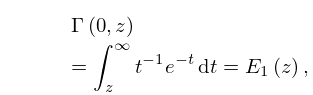
21: 16.7 Relations to Other Functions

… ►For

\mathit{3j}

\mathit{6j}

\mathit{9j}

symbols see Chapter 34. Further representations of special functions in terms of

{{}_{p}F_{q}}

functions are given in Luke (1969a, §§6.2–6.3), and an extensive list of

{{}_{q+1}F_{q}}

functions with rational numbers as parameters is given in Krupnikov and Kölbig (1997).

22: 10 Bessel Functions

…

23: 23 Weierstrass Elliptic and Modular
Functions

…

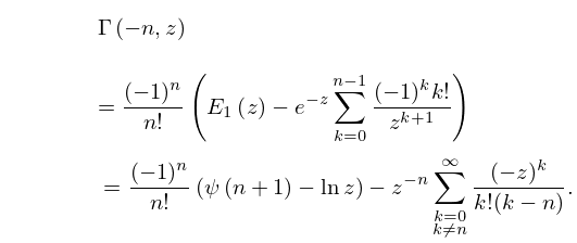
24: 8.4 Special Values

… ►For

\operatorname{erf}\left(z\right)

\operatorname{erfc}\left(z\right)

, and

F\left(z\right)

, see §§7.2(i), 7.2(ii). For

E_{n}\left(z\right)

see §8.19(i). … ►

8.4.4

\Gamma\left(0,z\right)=\int_{z}^{\infty}t^{-1}e^{-t}\,\mathrm{d}t=E_{1}\left(z% \right),

ⓘ

Symbols:: $\,\mathrm{d}\NVar{x}$ : differential of $x$ , $\mathrm{e}$ : base of natural logarithm, $E_{1}\left(\NVar{z}\right)$ : exponential integral, $\Gamma\left(\NVar{a},\NVar{z}\right)$ : incomplete gamma function, $\int$ : integral and $z$ : complex variable
A&S Ref:: 6.5.15
Permalink:: http://dlmf.nist.gov/8.4.E4
Encodings:: pMML, png, TeX
See also:: Annotations for §8.4 and Ch.8

… ►

8.4.13

\Gamma\left(1-n,z\right)=z^{1-n}E_{n}\left(z\right),

ⓘ

Symbols:: $E_{\NVar{p}}\left(\NVar{z}\right)$ : generalized exponential integral, $\Gamma\left(\NVar{a},\NVar{z}\right)$ : incomplete gamma function, $z$ : complex variable and $n$ : nonnegative integer
Referenced by:: §8.19(iv)
Permalink:: http://dlmf.nist.gov/8.4.E13
Encodings:: pMML, png, TeX
See also:: Annotations for §8.4 and Ch.8

… ►

8.4.15

\Gamma\left(-n,z\right)=\frac{(-1)^{n}}{n!}\left(E_{1}\left(z\right)-e^{-z}% \sum_{k=0}^{n-1}\frac{(-1)^{k}k!}{z^{k+1}}\right)=\frac{(-1)^{n}}{n!}\left(% \psi\left(n+1\right)-\ln z\right)-z^{-n}\sum_{\begin{subarray}{c}k=0\\ k\neq n\end{subarray}}^{\infty}\frac{(-z)^{k}}{k!(k-n)}.

ⓘ

Symbols:: $\psi\left(\NVar{z}\right)$ : psi (or digamma) function, $\mathrm{e}$ : base of natural logarithm, $E_{1}\left(\NVar{z}\right)$ : exponential integral, $!$ : factorial (as in $n!$ ), $\Gamma\left(\NVar{a},\NVar{z}\right)$ : incomplete gamma function, $\ln\NVar{z}$ : principal branch of logarithm function, $z$ : complex variable, $k$ : nonnegative integer and $n$ : nonnegative integer
A&S Ref:: 6.5.19
Referenced by:: §8.19(iii), §8.19(iv), §8.4
Permalink:: http://dlmf.nist.gov/8.4.E15
Encodings:: pMML, png, TeX
See also:: Annotations for §8.4 and Ch.8

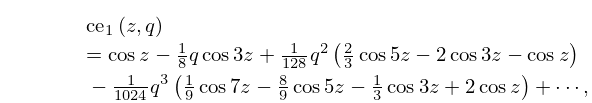
25: 28.6 Expansions for Small $q$

… ►Leading terms of the of the power series for

m=7,8,9,\dots

are: … ►Numerical values of the radii of convergence

\rho_{n}^{(j)}

of the power series (28.6.1)–(28.6.14) for

n=0,1,\dots,9

are given in Table 28.6.1. … ►where

k

is the unique root of the equation

2E\left(k\right)=K\left(k\right)

in the interval

(0,1)

, and

k^{\prime}=\sqrt{1-k^{2}}

. For

E\left(k\right)

and

K\left(k\right)

see §19.2(ii). … ►

28.6.22

\operatorname{ce}_{1}\left(z,q\right)=\cos z-\tfrac{1}{8}q\cos 3z+\tfrac{1}{12% 8}q^{2}\left(\tfrac{2}{3}\cos 5z-2\cos 3z-\cos z\right)-\tfrac{1}{1024}q^{3}% \left(\tfrac{1}{9}\cos 7z-\tfrac{8}{9}\cos 5z-\tfrac{1}{3}\cos 3z+2\cos z% \right)+\cdots,

ⓘ

Symbols:: $\operatorname{ce}_{\NVar{n}}\left(\NVar{z},\NVar{q}\right)$ : Mathieu function, $\cos\NVar{z}$ : cosine function, $q=h^{2}$ : parameter and $z$ : complex variable
Permalink:: http://dlmf.nist.gov/28.6.E22
Encodings:: pMML, png, TeX
See also:: Annotations for §28.6(ii), §28.6 and Ch.28

…

26: 3.5 Quadrature

… ►If

f\in C^{2m+2}[a,b]

, then the remainder

E_{n}(f)

in (3.5.2) can be expanded in the form … ►About

2^{9}=512

function evaluations are needed. … ►with weight function

w(x)

, is one for which

E_{n}(f)=0

whenever

f

is a polynomial of degree

\leq n-1

. The nodes

x_{1},x_{2},\dots,x_{n}

are prescribed, and the weights

w_{k}

and error term

E_{n}(f)

are found by integrating the product of the Lagrange interpolation polynomial of degree

n-1

and

w(x)

. … ►where

E_{n}(f)=0

f(\zeta)

is a polynomial of degree

\leq 2n-1

1/\zeta

. …

27: 34.8 Approximations for Large Parameters

§34.8 Approximations for Large Parameters

►For large values of the parameters in the

\mathit{3j}

\mathit{6j}

, and

\mathit{9j}

symbols, different asymptotic forms are obtained depending on which parameters are large. … ►For approximations for the

\mathit{3j}

\mathit{6j}

, and

\mathit{9j}

symbols with error bounds see Flude (1998), Chen et al. (1999), and Watson (1999): these references also cite earlier work.

28: 36.7 Zeros

… ►Inside the cusp, that is, for

x^{2}<8|y|^{3}/27

, the zeros form pairs lying in curved rows. … ►Just outside the cusp, that is, for

x^{2}>8|y|^{3}/27

, there is a single row of zeros on each side. … ►The zeros are lines in

\mathbf{x}=(x,y,z)

space where

\operatorname{ph}\Psi^{(\mathrm{E})}\left(\mathbf{x}\right)

is undetermined. …Near

z=z_{n}

, and for small

x

and

y

, the modulus

|\Psi^{(\mathrm{E})}\left(\mathbf{x}\right)|

has the symmetry of a lattice with a rhombohedral unit cell that has a mirror plane and an inverse threefold axis whose

z

and

x

repeat distances are given by …The rings are almost circular (radii close to

(\Delta x)/9

and varying by less than 1%), and almost flat (deviating from the planes

z_{n}

by at most

(\Delta z)/36

). …

29: 3.6 Linear Difference Equations

… ►The Weber function

\mathbf{E}_{n}\left(1\right)

satisfies …Thus the asymptotic behavior of the particular solution

\mathbf{E}_{n}\left(1\right)

is intermediate to those of the complementary functions

J_{n}\left(1\right)

and

Y_{n}\left(1\right)

; moreover, the conditions for Olver’s algorithm are satisfied. We apply the algorithm to compute

\mathbf{E}_{n}\left(1\right)

to 8S for the range

n=1,2,\dots,10

, beginning with the value

\mathbf{E}_{0}\left(1\right)=-0.56865\;\,663

obtained from the Maclaurin series expansion (§11.10(iii)). … ►The values of

w_{n}

for

n=1,2,\dots,10

are the wanted values of

\mathbf{E}_{n}\left(1\right)

. (It should be observed that for

n>10

, however, the

w_{n}

are progressively poorer approximations to

\mathbf{E}_{n}\left(1\right)

: the underlined digits are in error.) …

30: 2.11 Remainder Terms; Stokes Phenomenon

… ►The procedure followed in §2.11(ii) enabled

E_{p}\left(z\right)

to be computed with as much accuracy in the sector

\pi\leq\operatorname{ph}z\leq 3\pi

as the original expansion (2.11.6) in

|\operatorname{ph}z|\leq\pi

. … ►Owing to the factor

e^{-\rho}

, that is,

e^{-|z|}

in (2.11.13),

F_{n+p}\left(z\right)

is uniformly exponentially small compared with

E_{p}\left(z\right)

. For this reason the expansion of

E_{p}\left(z\right)

|\operatorname{ph}z|\leq\pi-\delta

supplied by (2.11.8), (2.11.10), and (2.11.13) is said to be exponentially improved. … ►However, to enjoy the resurgence property (§2.7(ii)) we often seek instead expansions in terms of the

F

-functions introduced in §2.11(iii), leaving the connection of the error-function type behavior as an implicit consequence of this property of the

F

-functions. In this context the

F

-functions are called terminants, a name introduced by Dingle (1973). …

21—30 of 625 matching pages

21: 16.7 Relations to Other Functions

22: 10 Bessel Functions

23: 23 Weierstrass Elliptic and Modular Functions

24: 8.4 Special Values

25: 28.6 Expansions for Small q

26: 3.5 Quadrature

27: 34.8 Approximations for Large Parameters

§34.8 Approximations for Large Parameters

28: 36.7 Zeros

29: 3.6 Linear Difference Equations

30: 2.11 Remainder Terms; Stokes Phenomenon

23: 23 Weierstrass Elliptic and Modular
Functions

25: 28.6 Expansions for Small $q$