.%E4%BB%8A%E5%B9%B4%E4%B8%96%E7%95%8C%E6%9D%AF%E5%AF%B9%E9%98%B5__%E3%80%8Ewn4.com_%E3%80%8F_%E5%B7%B4%E8%A5%BF%E4%B8%96%E7%95%8C%E6%9D%AF%E6%A2%85%E8%A5%BF%E9%87%91%E7%90%83%E5%A5%96_w6n2c9o_2022%E5%B9%B411%E6%9C%8830%E6%97%A58%E6%97%B67%E5%88%86_lvhhtouai.com

SearchAdvancedHelp

(0.084 seconds)

11—20 of 827 matching pages

11: 23.4 Graphics

… ►

►►

Figure 23.4.1: $\mathrm{\wp }(x;g_2,0)$ for $0\le x\le 9$, $g_2$ = 0. …8. … Magnify

►

►►

Figure 23.4.2: $\mathrm{\wp }(x;0,g_3)$ for $0\le x\le 9$, $g_3$ = 0. …8. … Magnify

►

►►

Figure 23.4.3: $\zeta (x;g_2,0)$ for $0\le x\le 8$, $g_2$ = 0. …8. … Magnify

►

►►

Figure 23.4.4: $\zeta (x;0,g_3)$ for $0\le x\le 8$, $g_3$ = 0. …8. … Magnify

►

►►

Figure 23.4.5: $\sigma (x;g_2,0)$ for $-5\le x\le 5$, $g_2$ = 0. …8. … Magnify

…

12: 23.1 Special Notation

… ►The main functions treated in this chapter are the Weierstrass $\mathrm{\wp }$-function $\mathrm{\wp }\left(z\right)=\mathrm{\wp }\left(z|𝕃\right)=\mathrm{\wp }(z;g_2,g_3)$; the Weierstrass zeta function $\zeta \left(z\right)=\zeta \left(z|𝕃\right)=\zeta (z;g_2,g_3)$; the Weierstrass sigma function $\sigma \left(z\right)=\sigma \left(z|𝕃\right)=\sigma (z;g_2,g_3)$; the elliptic modular function $\lambda \left(\tau \right)$; Klein’s complete invariant $J\left(\tau \right)$; Dedekind’s eta function $\eta \left(\tau \right)$. … ►Whittaker and Watson (1927) requires only $\mathrm{\Im }\left({\omega }_3/{\omega }_1\right)\ne 0$, instead of $\mathrm{\Im }\left({\omega }_3/{\omega }_1\right)>0$. Abramowitz and Stegun (1964, Chapter 18) considers only rectangular and rhombic lattices (§23.5); ${\omega }_1$, ${\omega }_3$ are replaced by $\omega$, ${\omega }^{\prime }$ for the former and by ${\omega }_2$, ${\omega }^{\prime }$ for the latter. Silverman and Tate (1992) and Koblitz (1993) replace $2{\omega }_1$ and $2{\omega }_3$ by ${\omega }_1$ and ${\omega }_3$, respectively. Walker (1996) normalizes $2{\omega }_1=1$, $2{\omega }_3=\tau$, and uses homogeneity (§23.10(iv)). …

13: 23.6 Relations to Other Functions

… ►In this subsection $2{\omega }_1$, $2{\omega }_3$ are any pair of generators of the lattice $𝕃$, and the lattice roots $e_1$, $e_2$, $e_3$ are given by (23.3.9). …With $z=\pi u/(2{\omega }_1)$, … ►Again, in Equations (23.6.16)–(23.6.26), $2{\omega }_1,2{\omega }_3$ are any pair of generators of the lattice $𝕃$ and $e_1,e_2,e_3$ are given by (23.3.9). … ►Also, ${𝕃}_1$, ${𝕃}_2$, ${𝕃}_3$ are the lattices with generators $(4K,2\mathrm{i}{K}^{\prime })$, $(2K-2\mathrm{i}{K}^{\prime },2K+2\mathrm{i}{K}^{\prime })$, $(2K,4\mathrm{i}{K}^{\prime })$, respectively. 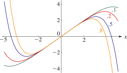… ►Let $z$ be on the perimeter of the rectangle with vertices $0,2{\omega }_1,2{\omega }_1+2{\omega }_3,2{\omega }_3$. …

14: 23.8 Trigonometric Series and Products

… ►If $q={\mathrm{e}}^{\mathrm{i}\pi {\omega }_3/{\omega }_1}$, , and $z\notin 𝕃$, then … ►When $z\notin 𝕃$, ►

23.8.3 $$\mathrm{\wp }\left(z\right)=-\frac{{\eta }_1}{{\omega }_1}+\frac{{\pi }^2}{4{\omega }_1^2}\sum _{n=-\mathrm{\infty }}^{\mathrm{\infty }}{\csc }^2\left(\frac{\pi (z+2n{\omega }_3)}{2{\omega }_1}\right),$$

ⓘ

Symbols:

$\mathrm{\wp }\left(z\right)$ (= $\mathrm{\wp }\left(z|𝕃\right)$ = $\mathrm{\wp }(z;g_2,g_3)$): Weierstrass $\mathrm{\wp }$-function, $\pi$: the ratio of the circumference of a circle to its diameter, $\csc z$: cosecant function, $𝕃$: lattice, $n$: integer, $z$: complex, ${\omega }_1$, ${\omega }_3$, ${\omega }_2=-{\omega }_1-{\omega }_3$: lattice generators and ${\eta }_j$: complex number

Permalink:

http://dlmf.nist.gov/23.8.E3

Encodings:

pMML, png, TeX

See also:

Annotations for §23.8(ii), §23.8 and Ch.23

… ► …with similar results for ${\eta }_2$ and ${\eta }_3$ obtainable by use of (23.2.14). …

15: 23.21 Physical Applications

… ►The Weierstrass function $\mathrm{\wp }$ plays a similar role for cubic potentials in canonical form $g_3+g_{2}x-4x^3$. … ►For applications to soliton solutions of the Korteweg–de Vries (KdV) equation see McKean and Moll (1999, p. 91), Deconinck and Segur (2000), and Walker (1996, §8.1). … ►where $x,y,z$ are the corresponding Cartesian coordinates and $e_1$, $e_2$, $e_3$ are constants. … ►

23.21.3 $$f(\rho )=2{\left((\rho -e_1)(\rho -e_2)(\rho -e_3)\right)}^{1/2}.$$

ⓘ

Symbols:

$e_j$: Weierstrass lattice roots, $𝕃$: lattice, $\rho$: roots and $f(\rho )$: function

Permalink:

http://dlmf.nist.gov/23.21.E3

Encodings:

pMML, png, TeX

See also:

Annotations for §23.21(iii), §23.21 and Ch.23

►Another form is obtained by identifying $e_1$, $e_2$, $e_3$ as lattice roots (§23.3(i)), and setting …

16: 8 Incomplete Gamma and Related
Functions

Chapter 8 Incomplete Gamma and Related Functions

…

17: 23.20 Mathematical Applications

… ►It follows from the addition formula (23.10.1) that the points $P_j=P(z_j)$, $j=1,2,3$, have zero sum iff $z_1+z_2+z_3\in 𝕃$, so that addition of points on the curve $C$ corresponds to addition of parameters $z_j$ on the torus $ℂ/𝕃$; see McKean and Moll (1999, §§2.11, 2.14). … ►Given $P$, calculate $2P$, $4P$, $8P$ by doubling as above. …If any of $2P$, $4P$, $8P$ is not an integer, then the point has infinite order. Otherwise observe any equalities between $P$, $2P$, $4P$, $8P$, and their negatives. The order of a point (if finite and not already determined) can have only the values 3, 5, 6, 7, 9, 10, or 12, and so can be found from $2P=-P$, $4P=-P$, $4P=-2P$, $8P=P$, $8P=-P$, $8P=-2P$, or $8P=-4P$. …

18: 1.2 Elementary Algebra

… ►The transpose of $𝐀$ = $[a_{ij}]$ is the $n\times m$ matrix … ►For matrices $𝐀$, $𝐁$ and $𝐂$ of the same dimensions, … ► $𝐀$ is an upper or lower triangular matrix if all $a_{ij}$ vanish for $i>j$ or , respectively. … ►If $det(𝐀)=0$ then $𝐀𝐁=𝐀𝐂$ does not imply that $𝐁=𝐂$; if $det(𝐀)\ne 0$, then $𝐁=𝐂$, as both sides may be multiplied by ${𝐀}^{-1}$. … ►The trace of $𝐀=[a_{ij}]$ is …

19: 23.5 Special Lattices

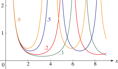
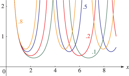
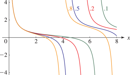
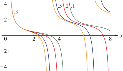
… ►The Weierstrass functions take real values on the real axis iff the lattice is fixed under complex conjugation: $𝕃=\overline{𝕃}$; equivalently, when $g_2,g_3\in ℝ$. … ►This occurs when both ${\omega }_1$ and ${\omega }_3/\mathrm{i}$ are real and positive. Then $\mathrm{\Delta }>0$ and the parallelogram with vertices at $0$, $2{\omega }_1$, $2{\omega }_1+2{\omega }_3$, $2{\omega }_3$ is a rectangle. ►In this case the lattice roots $e_1$, $e_2$, and $e_3$ are real and distinct. …Also, $e_2$ and $g_3$ have opposite signs unless ${\omega }_3=\mathrm{i}{\omega }_1$, in which event both are zero. …

20: 3.2 Linear Algebra

… ►Forward elimination for solving $𝐀𝐱=𝐟$ then becomes $y_1=f_1$, … ►The $p$-norm of a matrix $𝐀=[a_{jk}]$ is …The cases $p=1,2$, and $\mathrm{\infty }$ are the most important: … ►has the same eigenvalues as $𝐀$. … ►Many methods are available for computing eigenvalues; see Golub and Van Loan (1996, Chapters 7, 8), Trefethen and Bau (1997, Chapter 5), and Wilkinson (1988, Chapters 8, 9).