抢庄牛牛3D游戏大厅,网上抢庄牛牛3D游戏规则,【复制打开网址：33kk55.com】正规博彩平台,在线赌博平台,抢庄牛牛3D游戏玩法介绍,真人抢庄牛牛3D游戏规则,网上真人棋牌游戏平台,真人博彩游戏平台网址YBsCyXMBsMAyNMBM

(0.005 seconds)

21—30 of 590 matching pages

21: 18.38 Mathematical Applications

… ►For these results and applications in approximation theory see §3.11(ii) and Mason and Handscomb (2003, Chapter 3), Cheney (1982, p. 108), and Rivlin (1969, p. 31). … ►

$3j$ and $6j$ Symbols

… ► … ►The abstract associative algebra with generators

K_{0},K_{1},K_{2}

and relations (18.38.4), (18.38.6) and with the constants

B,C_{0},C_{1},D_{0},D_{1}

in (18.38.6) not yet specified, is called the Zhedanov algebra or Askey–Wilson algebra AW(3). …See Zhedanov (1991), Granovskiĭ et al. (1992, §3), Koornwinder (2007a, §2) and Terwilliger (2011). …

22: 21.6 Products

… ►

21.6.2

\mathcal{D}=|\mathbf{T}^{\mathrm{T}}{\mathbb{Z}}^{h}/(\mathbf{T}^{\mathrm{T}}{% \mathbb{Z}}^{h}\cap{\mathbb{Z}}^{h})|,

ⓘ

Defines:: $\mathcal{D}$ : number of elements (locally)
Symbols:: $\mathbb{Z}$ : set of all integers, $\cap$ : intersection, $\NVar{\mathbf{A}}^{\mathrm{T}}$ : transpose of matrix and $h$ : positive integer
Permalink:: http://dlmf.nist.gov/21.6.E2
Encodings:: pMML, png, TeX
See also:: Annotations for §21.6(i), §21.6 and Ch.21

►that is,

\mathcal{D}

is the number of elements in the set containing all

h

-dimensional vectors obtained by multiplying

\mathbf{T}^{\mathrm{T}}

on the right by a vector with integer elements. … ►

21.6.3

\prod_{j=1}^{h}\theta\left(\sum_{k=1}^{h}T_{jk}\mathbf{z}_{k}\middle|% \boldsymbol{{\Omega}}\right)=\frac{1}{\mathcal{D}^{g}}\sum_{\mathbf{A}\in% \mathcal{K}}\sum_{\mathbf{B}\in\mathcal{K}}e^{2\pi i\operatorname{tr}\left[% \frac{1}{2}\mathbf{A}^{\mathrm{T}}\boldsymbol{{\Omega}}\mathbf{A}+\mathbf{A}^{% \mathrm{T}}[\mathbf{Z}+\mathbf{B}]\right]}\*\prod_{j=1}^{h}\theta\left(\mathbf% {z}_{j}+\boldsymbol{{\Omega}}\mathbf{a}_{j}+\mathbf{b}_{j}\middle|\boldsymbol{% {\Omega}}\right),

… ►

21.6.4

\prod_{j=1}^{h}\theta\genfrac{[}{]}{0.0pt}{}{\sum_{k=1}^{h}T_{jk}\mathbf{c}_{k% }}{\sum_{k=1}^{h}T_{jk}\mathbf{d}_{k}}\left(\sum_{k=1}^{h}T_{jk}\mathbf{z}_{k}% \middle|\boldsymbol{{\Omega}}\right)=\frac{1}{\mathcal{D}^{g}}\sum_{\mathbf{A}% \in\mathcal{K}}\sum_{\mathbf{B}\in\mathcal{K}}e^{-2\pi i\sum_{j=1}^{h}\mathbf{% b}_{j}\cdot\mathbf{c}_{j}}\prod_{j=1}^{h}\theta\genfrac{[}{]}{0.0pt}{}{\mathbf% {a}_{j}+\mathbf{c}_{j}}{\mathbf{b}_{j}+\mathbf{d}_{j}}\left(\mathbf{z}_{j}% \middle|\boldsymbol{{\Omega}}\right),

ⓘ

Symbols:: $\theta\genfrac{[}{]}{0.0pt}{}{\NVar{\boldsymbol{{\alpha}}}}{\NVar{\boldsymbol{% {\beta}}}}\left(\NVar{\mathbf{z}}\middle|\NVar{\boldsymbol{{\Omega}}}\right)$ : Riemann theta function with characteristics, $\pi$ : the ratio of the circumference of a circle to its diameter, $\in$ : element of, $\mathrm{e}$ : base of natural logarithm, $\mathrm{i}$ : imaginary unit, $g$ : positive integer, $h$ : positive integer, $\boldsymbol{{\Omega}}$ : a Riemann matrix, $T_{jk}$ : element, $\mathcal{K}$ : set of matrices and $\mathcal{D}$ : number of elements
Permalink:: http://dlmf.nist.gov/21.6.E4
Encodings:: pMML, png, TeX
See also:: Annotations for §21.6(i), §21.6 and Ch.21

… ►

21.6.7

\theta\genfrac{[}{]}{0.0pt}{}{\tfrac{1}{2}[\mathbf{c}_{1}+\mathbf{c}_{2}+% \mathbf{c}_{3}+\mathbf{c}_{4}]}{\tfrac{1}{2}[\mathbf{d}_{1}+\mathbf{d}_{2}+% \mathbf{d}_{3}+\mathbf{d}_{4}]}\left(\frac{\mathbf{x}+\mathbf{y}+\mathbf{u}+% \mathbf{v}}{2}\middle|\boldsymbol{{\Omega}}\right)\theta\genfrac{[}{]}{0.0pt}{% }{\tfrac{1}{2}[\mathbf{c}_{1}+\mathbf{c}_{2}-\mathbf{c}_{3}-\mathbf{c}_{4}]}{% \tfrac{1}{2}[\mathbf{d}_{1}+\mathbf{d}_{2}-\mathbf{d}_{3}-\mathbf{d}_{4}]}% \left(\frac{\mathbf{x}+\mathbf{y}-\mathbf{u}-\mathbf{v}}{2}\middle|\boldsymbol% {{\Omega}}\right)\*\theta\genfrac{[}{]}{0.0pt}{}{\tfrac{1}{2}[\mathbf{c}_{1}-% \mathbf{c}_{2}+\mathbf{c}_{3}-\mathbf{c}_{4}]}{\tfrac{1}{2}[\mathbf{d}_{1}-% \mathbf{d}_{2}+\mathbf{d}_{3}-\mathbf{d}_{4}]}\left(\frac{\mathbf{x}-\mathbf{y% }+\mathbf{u}-\mathbf{v}}{2}\middle|\boldsymbol{{\Omega}}\right)\theta\genfrac{% [}{]}{0.0pt}{}{\tfrac{1}{2}[\mathbf{c}_{1}-\mathbf{c}_{2}-\mathbf{c}_{3}+% \mathbf{c}_{4}]}{\tfrac{1}{2}[\mathbf{d}_{1}-\mathbf{d}_{2}-\mathbf{d}_{3}+% \mathbf{d}_{4}]}\left(\frac{\mathbf{x}-\mathbf{y}-\mathbf{u}+\mathbf{v}}{2}% \middle|\boldsymbol{{\Omega}}\right)\\ =\frac{1}{2^{g}}\sum_{\boldsymbol{{\alpha}}\in\frac{1}{2}{\mathbb{Z}}^{g}/{% \mathbb{Z}}^{g}}\,\sum_{\boldsymbol{{\beta}}\in\frac{1}{2}{\mathbb{Z}}^{g}/{% \mathbb{Z}}^{g}}e^{-2\pi i\boldsymbol{{\beta}}\cdot[\mathbf{c}_{1}+\mathbf{c}_% {2}+\mathbf{c}_{3}+\mathbf{c}_{4}]}\*\theta\genfrac{[}{]}{0.0pt}{}{\mathbf{c}_% {1}+\boldsymbol{{\alpha}}}{\mathbf{d}_{1}+\boldsymbol{{\beta}}}\left(\mathbf{x% }\middle|\boldsymbol{{\Omega}}\right)\theta\genfrac{[}{]}{0.0pt}{}{\mathbf{c}_% {2}+\boldsymbol{{\alpha}}}{\mathbf{d}_{2}+\boldsymbol{{\beta}}}\left(\mathbf{y% }\middle|\boldsymbol{{\Omega}}\right)\theta\genfrac{[}{]}{0.0pt}{}{\mathbf{c}_% {3}+\boldsymbol{{\alpha}}}{\mathbf{d}_{3}+\boldsymbol{{\beta}}}\left(\mathbf{u% }\middle|\boldsymbol{{\Omega}}\right)\theta\genfrac{[}{]}{0.0pt}{}{\mathbf{c}_% {4}+\boldsymbol{{\alpha}}}{\mathbf{d}_{4}+\boldsymbol{{\beta}}}\left(\mathbf{v% }\middle|\boldsymbol{{\Omega}}\right).

ⓘ

Symbols:: $\theta\genfrac{[}{]}{0.0pt}{}{\NVar{\boldsymbol{{\alpha}}}}{\NVar{\boldsymbol{% {\beta}}}}\left(\NVar{\mathbf{z}}\middle|\NVar{\boldsymbol{{\Omega}}}\right)$ : Riemann theta function with characteristics, $\pi$ : the ratio of the circumference of a circle to its diameter, $\in$ : element of, $\mathrm{e}$ : base of natural logarithm, $\mathrm{i}$ : imaginary unit, $\mathbb{Z}$ : set of all integers, $g$ : positive integer, $\boldsymbol{{\Omega}}$ : a Riemann matrix, $\boldsymbol{{\alpha}}$ : $g$ -dimensional vector and $\boldsymbol{{\beta}}$ : $g$ -dimensional vector
Permalink:: http://dlmf.nist.gov/21.6.E7
Encodings:: pMML, png, TeX
See also:: Annotations for §21.6(i), §21.6(i), §21.6 and Ch.21

…

23: 19.34 Mutual Inductance of Coaxial Circles

… ►

a_{3}=h^{2}+a^{2}+b^{2},

… ►

19.34.3

2abI(\mathbf{e}_{5})=a_{3}I(\boldsymbol{{0}})-I(\mathbf{e}_{3})=a_{3}I(% \boldsymbol{{0}})-r_{+}^{2}r_{-}^{2}I(-\mathbf{e}_{3})=2ab(I(\boldsymbol{{0}})% -r_{-}^{2}I(\mathbf{e}_{1}-\mathbf{e}_{3})),

ⓘ

Symbols:: $I(\mathbf{m})$ : integral and $r_{\pm}$
Permalink:: http://dlmf.nist.gov/19.34.E3
Encodings:: pMML, png, TeX
See also:: Annotations for §19.34 and Ch.19

… ►

19.34.4

r_{\pm}^{2}=a_{3}\pm 2ab=h^{2}+(a\pm b)^{2}

ⓘ

Symbols:: $h$ : distance and $r_{\pm}$
Permalink:: http://dlmf.nist.gov/19.34.E4
Encodings:: pMML, png, TeX
See also:: Annotations for §19.34 and Ch.19

… ►Application of (19.29.4) and (19.29.7) with

\alpha=1

a_{\beta}+b_{\beta}t=1-t

\delta=3

, and

a_{\gamma}+b_{\gamma}t=1

yields ►

19.34.5

\frac{3{c}^{2}}{8\pi ab}M=3R_{F}\left(0,r_{+}^{2},r_{-}^{2}\right)-2r_{-}^{2}R% _{D}\left(0,r_{+}^{2},r_{-}^{2}\right),

ⓘ

Symbols:: $R_{D}\left(\NVar{x},\NVar{y},\NVar{z}\right)$ : elliptic integral symmetric in only two variables, $R_{F}\left(\NVar{x},\NVar{y},\NVar{z}\right)$ : symmetric elliptic integral of first kind, $\pi$ : the ratio of the circumference of a circle to its diameter, $M$ : mutual inductance and $r_{\pm}$
Permalink:: http://dlmf.nist.gov/19.34.E5
Encodings:: pMML, png, TeX
See also:: Annotations for §19.34 and Ch.19

…

24: 30.3 Eigenvalues

… ►

2\ell_{2}=-1-\frac{(2m-1)(2m+1)}{(2n-1)(2n+3)},

►

2\ell_{4}=\frac{(n-m-1)(n-m)(n+m-1)(n+m)}{(2n-3)(2n-1)^{3}(2n+1)}-\frac{(n-m+1% )(n-m+2)(n+m+1)(n+m+2)}{(2n+1)(2n+3)^{3}(2n+5)}.

… ►

30.3.11

\ell_{8}=2(4m^{2}-1)^{2}A+\frac{1}{16}B+\frac{1}{8}C+\frac{1}{2}D,

ⓘ

Symbols:: $m$ : nonnegative integer, $\ell_{j}$ : coefficients, $A$ , $B$ , $C$ and $D$
Permalink:: http://dlmf.nist.gov/30.3.E11
Encodings:: pMML, png, TeX
See also:: Annotations for §30.3(iv), §30.3 and Ch.30

… ►

B=\frac{(n-m-3)(n-m-2)(n-m-1)(n-m)(n+m-3)(n+m-2)(n+m-1)(n+m)}{(2n-7)(2n-5)^{2}% (2n-3)^{3}(2n-1)^{4}(2n+1)}-\frac{(n-m+1)(n-m+2)(n-m+3)(n-m+4)(n+m+1)(n+m+2)(n% +m+3)(n+m+4)}{(2n+1)(2n+3)^{4}(2n+5)^{3}(2n+7)^{2}(2n+9)},

… ►

D=\frac{(n-m-1)(n-m)(n-m+1)(n-m+2)(n+m-1)(n+m)(n+m+1)(n+m+2)}{(2n-3)(2n-1)^{4}% (2n+1)^{2}(2n+3)^{4}(2n+5)}.

…

25: 1.3 Determinants, Linear Operators, and Spectral Expansions

… ►For

n=3

: … ►

1.3.15

\begin{vmatrix}a_{1}&a_{2}&\cdots&a_{n}\\ a_{n}&a_{1}&\cdots&a_{n-1}\\ \vdots&\vdots&\ddots&\vdots\\ a_{2}&a_{3}&\cdots&a_{1}\end{vmatrix}=\prod^{n}_{k=1}(a_{1}+a_{2}\omega_{k}+a_% {3}\omega_{k}^{2}+\dots+a_{n}\omega_{k}^{n-1}),

ⓘ

Symbols:: $\det$ : determinant, $k$ : integer, $n$ : nonnegative integer and $\omega_{\NVar{j}}$ : roots of unity
Permalink:: http://dlmf.nist.gov/1.3.E15
Encodings:: pMML, png, TeX
See also:: Annotations for §1.3(ii), §1.3(ii), §1.3 and Ch.1

… ►Let

a_{j,k}

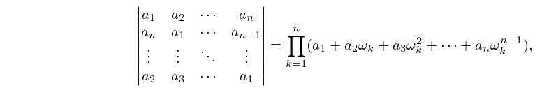
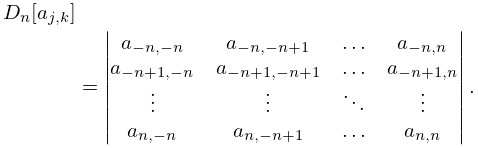
be defined for all integer values of

j

and

k

, and

D_{n}[a_{j,k}]

denote the

(2n+1)\times(2n+1)

determinant ►

1.3.18

D_{n}[a_{j,k}]=\begin{vmatrix}a_{-n,-n}&a_{-n,-n+1}&\dots&a_{-n,n}\\ a_{-n+1,-n}&a_{-n+1,-n+1}&\dots&a_{-n+1,n}\\ \vdots&\vdots&\ddots&\vdots\\ a_{n,-n}&a_{n,-n+1}&\dots&a_{n,n}\end{vmatrix}.

ⓘ

Defines:: $D_{\NVar{n}}[\NVar{a}_{\NVar{j},\NVar{k}}]$ : $(2\NVar{n}+1)\times(2\NVar{n}+1)$ determinant (locally)
Symbols:: $\det$ : determinant, $j$ : integer, $k$ : integer and $n$ : nonnegative integer
Permalink:: http://dlmf.nist.gov/1.3.E18
Encodings:: pMML, png, TeX
See also:: Annotations for §1.3(iii), §1.3 and Ch.1

►If

D_{n}[a_{j,k}]

tends to a limit

L

n\to\infty

, then we say that the infinite determinant

D_{\infty}[a_{j,k}]

converges and

D_{\infty}[a_{j,k}]=L

. …

26: 1.5 Calculus of Two or More Variables

… ►A function is continuous on a point set

D

if it is continuous at all points of

D

. … ►If

f(x,y)

is continuous, and

D

is the set … ►Similarly, if

D

is the set … ►If

D

can be represented in both forms (1.5.30) and (1.5.33), and

f(x,y)

is continuous on

D

, then … ►Infinite double integrals occur when

f(x,y)

becomes infinite at points in

D

or when

D

is unbounded. …

27: 19.25 Relations to Other Functions

… ►Equations (19.25.9)–(19.25.11) correspond to three (nonzero) choices for the last variable of

R_{D}

; see (19.21.7). … ►In (19.25.38) and (19.25.39)

j

k

\ell

is any permutation of the numbers

1,2,3

. … ►For these results and extensions to the Appell function

{F_{1}}

(§16.13) and Lauricella’s function

F_{D}

see Carlson (1963). (

{F_{1}}

and

F_{D}

are equivalent to the

R

-function of 3 and

n

variables, respectively, but lack full symmetry.) …

28: 24.2 Definitions and Generating Functions

… ►

Table 24.2.3: Bernoulli numbers

B_{n}=N/D

► ►►

$n$	$N$	$D$	$B_{n}$
…

► … ►

Table 24.2.5: Coefficients

b_{n,k}

of the Bernoulli polynomials

B_{n}\left(x\right)=\sum_{k=0}^{n}b_{n,k}x^{k}

► ►►►

	$k$
…
$3$	$0$	$\tfrac{1}{2}$	$-\tfrac{3}{2}$	$1$
…

► ►

Table 24.2.6: Coefficients

e_{n,k}

of the Euler polynomials

E_{n}\left(x\right)=\sum_{k=0}^{n}e_{n,k}x^{k}

► ►►►►

	$k$
…
$3$	$\tfrac{1}{4}$	$0$	$-\tfrac{3}{2}$	$1$
…
$6$	$0$	$-3$	$0$	$5$	$0$	$-3$	$1$
…

►

29: 31.2 Differential Equations

… ►where

2\omega_{1}

and

2\omega_{3}

with

\Im\left(\omega_{3}/\omega_{1}\right)>0

are generators of the lattice

\mathbb{L}

for

\wp\left(z|\mathbb{L}\right)

. … ►Lastly,

w(z)=(z-a)^{1-\epsilon}w_{3}(z)

satisfies (31.2.1) if

w_{3}

is a solution of (31.2.1) with transformed parameters

q_{3}=q+\gamma(1-\epsilon)

;

\alpha_{3}=\alpha+1-\epsilon

\beta_{3}=\beta+1-\epsilon

\epsilon_{3}=2-\epsilon

. By composing these three steps, there result

2^{3}=8

possible transformations of the dependent variable (including the identity transformation) that preserve the form of (31.2.1). … ►There are

4!=24

homographies

\tilde{z}(z)=(Az+B)/(Cz+D)

that take

0,1,a,\infty

to some permutation of

0,1,a^{\prime},\infty

, where

a^{\prime}

may differ from

a

. …If

\tilde{z}=\tilde{z}(z)

is one of the

4!-3!=18

homographies that do not map

\infty

\infty

, then an appropriate prefactor must be included on the right-hand side. …

30: 1.13 Differential Equations

… ►where

z\in D

, a simply-connected domain, and

f(z)

g(z)

are analytic in

D

, has an infinite number of analytic solutions in

D

. A solution becomes unique, for example, when

w

and

\ifrac{\mathrm{d}w}{\mathrm{d}z}

are prescribed at a point in

D

. … ►A fundamental pair can be obtained, for example, by taking any

z_{0}\in D

and requiring that … ►

u

and

z

belong to domains

U

and

D

respectively, the coefficients

f(u,z)

and

g(u,z)

are continuous functions of both variables, and for each fixed

u

(fixed

z

) the two functions are analytic in

z

(in

u

). … ►with

f(z)

g(z)

, and

r(z)

analytic in

D

has infinitely many analytic solutions in

D

. …

抢庄牛牛3D游戏大厅,网上抢庄牛牛3D游戏规则,【复制打开网址：33kk55.com】正规博彩平台,在线赌博平台,抢庄牛牛3D游戏玩法介绍,真人抢庄牛牛3D游戏规则,网上真人棋牌游戏平台,真人博彩游戏平台网址YBsCyXMBsMAyNMBM

21—30 of 590 matching pages

21: 18.38 Mathematical Applications

3 ⁢ j and 6 ⁢ j Symbols

22: 21.6 Products

23: 19.34 Mutual Inductance of Coaxial Circles

24: 30.3 Eigenvalues

25: 1.3 Determinants, Linear Operators, and Spectral Expansions

26: 1.5 Calculus of Two or More Variables

27: 19.25 Relations to Other Functions

28: 24.2 Definitions and Generating Functions

29: 31.2 Differential Equations

30: 1.13 Differential Equations

$3j$ and $6j$ Symbols