%E7%9C%9F%E4%BA%BA%E7%9C%9F%E9%92%B1%E6%A3%8B%E7%89%8C%E6%B8%B8%E6%88%8F%E5%A4%A7%E5%8E%85,%E7%BD%91%E4%B8%8A%E7%8E%B0%E9%87%91%E6%A3%8B%E7%89%8C%E6%B8%B8%E6%88%8F%E5%B9%B3%E5%8F%B0,%E3%80%90%E7%9C%9F%E4%BA%BA%E6%A3%8B%E7%89%8C%E5%AE%98%E6%96%B9%E7%BD%91%E7%AB%99%E2%88%B6789yule.com%E3%80%91%E7%BD%91%E4%B8%8A%E7%9C%9F%E9%92%B1%E6%A3%8B%E7%89%8C%E6%B8%B8%E6%88%8F%E5%A4%A7%E5%8E%85,%E5%9C%A8%E7%BA%BF%E6%A3%8B%E7%89%8C%E6%B8%B8%E6%88%8F%E7%BD%91%E7%AB%99,%E6%89%8B%E6%9C%BA%E6%A3%8B%E7%89%8Capp%E4%B8%8B%E8%BD%BD,%E6%A3%8B%E7%89%8C%E6%B8%B8%E6%88%8Fapp,%E6%A3%8B%E7%89%8C%E5%8D%9A%E5%BD%A9%E5%B9%B3%E5%8F%B0,%E3%80%90%E6%A3%8B%E7%89%8C%E6%B8%B8%E6%88%8F%E5%85%AC%E5%8F%B8%E2%88%B6789yule.com%E3%80%91%E7%BD%91%E5%9D%80ZEAE0CA0kAkn0BEB

SearchAdvancedHelp

(0.090 seconds)

11—20 of 612 matching pages

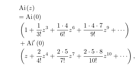
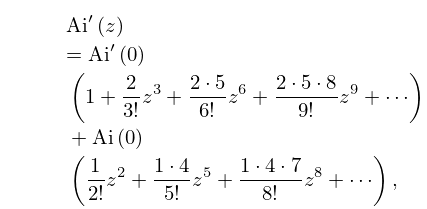
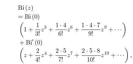
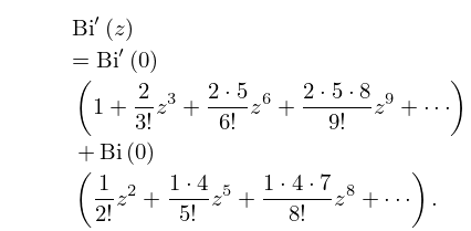
11: 9.4 Maclaurin Series

… ►

9.4.1 $$\mathrm{Ai}\left(z\right)=\mathrm{Ai}\left(0\right)\left(1+\frac{1}{3!}{z}^3+\frac{1\cdot 4}{6!}{z}^6+\frac{1\cdot 4\cdot 7}{9!}{z}^9+\mathrm{\cdots }\right)+{\mathrm{Ai}}^{\prime }\left(0\right)\left(z+\frac{2}{4!}{z}^4+\frac{2\cdot 5}{7!}{z}^7+\frac{2\cdot 5\cdot 8}{10!}{z}^{10}+\mathrm{\cdots }\right),$$

ⓘ

Symbols:

$\mathrm{Ai}\left(z\right)$: Airy function, $!$: factorial (as in $n!$) and $z$: complex variable

Source:

Olver (1997b, p. 54)

A&S Ref:

10.4.2 (with 10.4.4 and 10.4.5)

Permalink:

http://dlmf.nist.gov/9.4.E1

Encodings:

pMML, png, TeX

See also:

Annotations for §9.4 and Ch.9

►

9.4.2 $${\mathrm{Ai}}^{\prime }\left(z\right)={\mathrm{Ai}}^{\prime }\left(0\right)\left(1+\frac{2}{3!}{z}^3+\frac{2\cdot 5}{6!}{z}^6+\frac{2\cdot 5\cdot 8}{9!}{z}^9+\mathrm{\cdots }\right)+\mathrm{Ai}\left(0\right)\left(\frac{1}{2!}{z}^2+\frac{1\cdot 4}{5!}{z}^5+\frac{1\cdot 4\cdot 7}{8!}{z}^8+\mathrm{\cdots }\right),$$

ⓘ

Symbols:

$\mathrm{Ai}\left(z\right)$: Airy function, $!$: factorial (as in $n!$) and $z$: complex variable

Proof sketch:

Use methods of Olver (1997b, p. 54).

Permalink:

http://dlmf.nist.gov/9.4.E2

Encodings:

pMML, png, TeX

See also:

Annotations for §9.4 and Ch.9

►

9.4.3 $$\mathrm{Bi}\left(z\right)=\mathrm{Bi}\left(0\right)\left(1+\frac{1}{3!}{z}^3+\frac{1\cdot 4}{6!}{z}^6+\frac{1\cdot 4\cdot 7}{9!}{z}^9+\mathrm{\cdots }\right)+{\mathrm{Bi}}^{\prime }\left(0\right)\left(z+\frac{2}{4!}{z}^4+\frac{2\cdot 5}{7!}{z}^7+\frac{2\cdot 5\cdot 8}{10!}{z}^{10}+\mathrm{\cdots }\right),$$

ⓘ

Symbols:

$\mathrm{Bi}\left(z\right)$: Airy function, $!$: factorial (as in $n!$) and $z$: complex variable

Proof sketch:

Use methods of Olver (1997b, p. 54).

A&S Ref:

10.4.3 (with 10.4.4 and 10.4.5)

Referenced by:

(9.12.15)

Permalink:

http://dlmf.nist.gov/9.4.E3

Encodings:

pMML, png, TeX

See also:

Annotations for §9.4 and Ch.9

►

9.4.4 $${\mathrm{Bi}}^{\prime }\left(z\right)={\mathrm{Bi}}^{\prime }\left(0\right)\left(1+\frac{2}{3!}{z}^3+\frac{2\cdot 5}{6!}{z}^6+\frac{2\cdot 5\cdot 8}{9!}{z}^9+\mathrm{\cdots }\right)+\mathrm{Bi}\left(0\right)\left(\frac{1}{2!}{z}^2+\frac{1\cdot 4}{5!}{z}^5+\frac{1\cdot 4\cdot 7}{8!}{z}^8+\mathrm{\cdots }\right).$$

ⓘ

Symbols:

$\mathrm{Bi}\left(z\right)$: Airy function, $!$: factorial (as in $n!$) and $z$: complex variable

Proof sketch:

Use methods of Olver (1997b, p. 54).

Permalink:

http://dlmf.nist.gov/9.4.E4

Encodings:

pMML, png, TeX

See also:

Annotations for §9.4 and Ch.9

12: 18.8 Differential Equations

… ►

Table 18.8.1: Classical OP’s: differential equations $A(x)f^{\prime \prime }(x)+B(x)f^{\prime }(x)+C(x)f(x)+{\lambda }_{n}f(x)=0$.

► ►►►►►

#	$f(x)$	$A(x)$	$B(x)$	$C(x)$	${\lambda }_n$
…
4	$C_n^{(\lambda )}\left(x\right)$	$1-x^2$	$-(2\lambda +1)x$	$0$	$n(n+2\lambda )$
…
8	$L_n^{(\alpha )}\left(x\right)$	$x$	$\alpha +1-x$	$0$	$n$
9	${\mathrm{e}}^{-\frac{1}{2}{x}^2}{x}^{\alpha +\frac{1}{2}}{L}_n^{(\alpha )}\left(x^2\right)$	$1$	$0$	$-x^2+(\frac{1}{4}-{\alpha }^2)x^{-2}$	$4n+2\alpha +2$
…

►

…

13: Bibliography T

… ►

Improved error bounds for the Liouville-Green (or WKB) approximation. J. Math. Anal. Appl. 85 (1), pp. 79–89.

ⓘ

External Links:

ISSN 0022-247X, Document, MathReview (Klaus Deimling), ZentralBlatt

Referenced by:

§2.7(iii).

Encodings:

BibTeX

… ►

Asymptotic estimates of Stirling numbers. Stud. Appl. Math. 89 (3), pp. 233–243.

ⓘ

External Links:

ISSN 0022-2526, FullText, MathReview (E. Rodney Canfield), ZentralBlatt

Referenced by:

§26.8(vii).

Encodings:

BibTeX

… ►

Bernoulli polynomials old and new: Generalizations and asymptotics. CWI Quarterly 8 (1), pp. 47–66.

ⓘ

External Links:

ISSN 0922-5366, FullText, MathReview (Michael Hauss), ZentralBlatt

Referenced by:

§24.11, §24.16(i).

Encodings:

BibTeX

… ►

The universal Askey-Wilson algebra and DAHA of type $(C_1^{\vee },C_1)$ . SIGMA 9, pp. Paper 047, 40 pp..

ⓘ

External Links:

ISSN 1815-0659, Link, MathReview (Renato Álvarez-Nodarse), ZentralBlatt

Referenced by:

§18.38(iii).

Encodings:

BibTeX

… ►

Theory of the Fresnel integral. USSR Comput. Math. and Math. Phys. 9 (4), pp. 271–279.

ⓘ

Notes:

Translation of the paper in Zh. Vychisl. Mat. Mat. Fiz., Vol. 9, No. 4, 938-944, 1969

External Links:

Document, ZentralBlatt

Referenced by:

§7.13(iv).

Encodings:

BibTeX

14: 34.12 Physical Applications

§34.12 Physical Applications

►The angular momentum coupling coefficients ($\mathit{3}j$, $\mathit{6}j$, and $\mathit{9}j$ symbols) are essential in the fields of nuclear, atomic, and molecular physics. …$\mathit{3}j,\mathit{6}j$, and $\mathit{9}j$ symbols are also found in multipole expansions of solutions of the Laplace and Helmholtz equations; see Carlson and Rushbrooke (1950) and Judd (1976).

15: 24.2 Definitions and Generating Functions

… ►

$B_{2n+1}=0$ ,

… ►

24.2.4 $$B_n=B_n\left(0\right),$$

ⓘ

Symbols:

$B_n$: Bernoulli numbers, $B_n\left(x\right)$: Bernoulli polynomials and $n$: integer

A&S Ref:

23.1.2

Referenced by:

(25.11.7)

Permalink:

http://dlmf.nist.gov/24.2.E4

Encodings:

pMML, png, TeX

See also:

Annotations for §24.2(i), §24.2 and Ch.24

… ►

Table 24.2.4: Euler numbers $E_n$.

► ►►►

$n$	$E_n$
…
$8$	$1385$
…

►

►

Table 24.2.5: Coefficients $b_{n,k}$ of the Bernoulli polynomials $B_n\left(x\right)={\sum }_{k=0}^n{b}_{n,k}{x}^k$.

► ►►►

	$k$
$n$	$0$	$1$	$2$	$3$	$4$	$5$	$6$	$7$	$8$	$9$	$10$	$11$	$12$	$13$	$14$	$15$
…

►

►

Table 24.2.6: Coefficients $e_{n,k}$ of the Euler polynomials $E_n\left(x\right)={\sum }_{k=0}^n{e}_{n,k}{x}^k$.

► ►►►

	$k$
$n$	$0$	$1$	$2$	$3$	$4$	$5$	$6$	$7$	$8$	$9$	$10$	$11$	$12$	$13$	$14$	$15$
…

►

16: 2.10 Sums and Sequences

… ►For further information on $C$ see §5.17. … ►For extensions to $\alpha \le 0$, higher terms, and other examples, see Olver (1997b, Chapter 8). … ►where ${𝒞}_1,{𝒞}_2$ denote respectively the upper and lower halves of $𝒞$. … ►For generalizations and other examples see Olver (1997b, Chapter 8), Ford (1960), and Berndt and Evans (1984). … ►For examples see Olver (1997b, Chapters 8, 9). …

17: Bibliography

… ►

Evaluation of Coulomb wave functions along the transition line. Physical Rev. (2) 96, pp. 77–79.

ⓘ

External Links:

Document, MathReview (A. Erdélyi), ZentralBlatt

Referenced by:

§33.12(i).

Encodings:

BibTeX

… ►

Uniform asymptotic expansions for exponential integrals $E_n(x)$ and Bickley functions ${\mathrm{Ki}}_n(x)$ . ACM Trans. Math. Software 9 (4), pp. 467–479.

ⓘ

External Links:

ISSN 0098-3500, Document, MathReview (Marietta J. Tretter), ZentralBlatt

Referenced by:

§10.43(iii).

Encodings:

BibTeX

… ►

Theorems on generalized Dedekind sums. Pacific J. Math. 2 (1), pp. 1–9.

ⓘ

External Links:

MathReview (N. G. de Bruijn), ZentralBlatt

Referenced by:

(25.11.41), (25.11.42), §25.11(xii).

Encodings:

BibTeX

… ►

Numerical Tables for Angular Correlation Computations in $\alpha$-, $\beta$- and $\gamma$-Spectroscopy: $3j$-, $6j$-, $9j$-Symbols, F- and $\mathrm{\Gamma }$-Coefficients. Landolt-Börnstein Numerical Data and Functional Relationships in Science and Technology, Springer-Verlag.

ⓘ

External Links:

ISBN 978-3-540-04218-1

Referenced by:

§34.14.

Encodings:

BibTeX

… ►

A new treatment of the ellipsoidal wave equation. Proc. London Math. Soc. (3) 9, pp. 21–50.

ⓘ

External Links:

ISSN 0024-6115, Document, MathReview (J. Meixner), ZentralBlatt

Referenced by:

§29.11.

Encodings:

BibTeX

…

18: 14.33 Tables

… ►

Abramowitz and Stegun (1964, Chapter 8) tabulates ${𝖯}_n\left(x\right)$ for $n=0(1)3,9,10$, $x=0(.01)1$, 5–8D; ${𝖯}_n^{\prime }\left(x\right)$ for $n=1(1)4,9,10$, $x=0(.01)1$, 5–7D; ${𝖰}_n\left(x\right)$ and ${𝖰}_n^{\prime }\left(x\right)$ for $n=0(1)3,9,10$, $x=0(.01)1$, 6–8D; $P_n\left(x\right)$ and $P_n^{\prime }\left(x\right)$ for $n=0(1)5,9,10$, $x=1(.2)10$, 6S; $Q_n\left(x\right)$ and $Q_n^{\prime }\left(x\right)$ for $n=0(1)3,9,10$, $x=1(.2)10$, 6S. (Here primes denote derivatives with respect to $x$.)

►

Zhang and Jin (1996, Chapter 4) tabulates ${𝖯}_n\left(x\right)$ for $n=2(1)5,10$, $x=0(.1)1$, 7D; ${𝖯}_n\left(\cos \theta \right)$ for $n=1(1)4,10$, $\theta =0(5^{\circ }){90}^{\circ }$, 8D; ${𝖰}_n\left(x\right)$ for $n=0(1)2,10$, $x=0(.1)0.9$, 8S; ${𝖰}_n\left(\cos \theta \right)$ for $n=0(1)3,10$, $\theta =0(5^{\circ }){90}^{\circ }$, 8D; ${𝖯}_n^m\left(x\right)$ for $m=1(1)4$, $n-m=0(1)2$, $n=10$, $x=0,0.5$, 8S; ${𝖰}_n^m\left(x\right)$ for $m=1(1)4$, $n=0(1)2,10$, 8S; ${𝖯}_{\nu }^m\left(\cos \theta \right)$ for $m=0(1)3$, $\nu =0(.25)5$, $\theta =0({15}^{\circ }){90}^{\circ }$, 5D; $P_n\left(x\right)$ for $n=2(1)5,10$, $x=1(1)10$, 7S; $Q_n\left(x\right)$ for $n=0(1)2,10$, $x=2(1)10$, 8S. Corresponding values of the derivative of each function are also included, as are 6D values of the first 5 $\nu$-zeros of ${𝖯}_{\nu }^m\left(\cos \theta \right)$ and of its derivative for $m=0(1)4$, $\theta ={10}^{\circ },{30}^{\circ },{150}^{\circ }$.

►

Belousov (1962) tabulates ${𝖯}_n^m\left(\cos \theta \right)$ (normalized) for $m=0(1)36$, $n-m=0(1)56$, $\theta =0({2.5}^{\circ }){90}^{\circ }$, 6D.

…

19: 26.7 Set Partitions: Bell Numbers

… ► $B\left(n\right)$ is the number of partitions of $\{1,2,\mathrm{\dots },n\}$. … ►

26.7.1 $$B\left(0\right)=1,$$

ⓘ

Symbols:

$B\left(n\right)$: Bell number

Permalink:

http://dlmf.nist.gov/26.7.E1

Encodings:

pMML, png, TeX

See also:

Annotations for §26.7(i), §26.7 and Ch.26

►

26.7.2 $$B\left(n\right)=\sum _{k=0}^{n}S(n,k),$$

ⓘ

Symbols:

$B\left(n\right)$: Bell number, $S(n,k)$: Stirling number of the second kind, $k$: nonnegative integer and $n$: nonnegative integer

Permalink:

http://dlmf.nist.gov/26.7.E2

Encodings:

pMML, png, TeX

See also:

Annotations for §26.7(i), §26.7 and Ch.26

… ►

26.7.6 $$B\left(n+1\right)=\sum _{k=0}^n\left(\genfrac{}{}{0.0pt}{}{n}{k}\right)B\left(k\right).$$

ⓘ

Symbols:

$B\left(n\right)$: Bell number, $\left(\genfrac{}{}{0.0pt}{}{m}{n}\right)$: binomial coefficient, $k$: nonnegative integer and $n$: nonnegative integer

Referenced by:

Erratum (V1.0.1) for Equation (26.7.6)

Permalink:

http://dlmf.nist.gov/26.7.E6

Encodings:

pMML, png, TeX

Errata (effective with 1.0.1):

Originally appeared with $B\left(n\right)$ in the summation, instead of $B\left(k\right)$:

$$B\left(n+1\right)=\sum _{k=0}^n\left(\genfrac{}{}{0.0pt}{}{n}{k}\right)B\left(n\right)$$

Reported 2010-11-07 by Layne Watson

See also:

Annotations for §26.7(iii), §26.7 and Ch.26

… ►For higher approximations to $B\left(n\right)$ as $n\to \mathrm{\infty }$ see de Bruijn (1961, pp. 104–108).

20: 16.24 Physical Applications

… ►

§16.24(iii) $\mathit{3}j$, $\mathit{6}j$, and $\mathit{9}j$ Symbols

… ►They can be expressed as ${}_3{}^{}F_2^{}$ functions with unit argument. …These are balanced ${}_4{}^{}F_3^{}$ functions with unit argument. Lastly, special cases of the $\mathit{9}j$ symbols are ${}_5{}^{}F_4^{}$ functions with unit argument. …