%E5%8D%9A%E5%BD%A9%E5%B9%B3%E5%8F%B0%E5%A4%A7%E5%85%A8,%E5%8D%9A%E5%BD%A9%E5%B9%B3%E5%8F%B0%E6%8E%92%E5%90%8D,%E7%BD%91%E4%B8%8A%E5%8D%9A%E5%BD%A9%E5%85%AC%E5%8F%B8,%E3%80%90%E5%8D%9A%E5%BD%A9%E7%BD%91%E5%9D%80%E2%88%B6789yule.com%E3%80%91%E5%85%A8%E7%90%83%E6%9C%80%E5%A4%A7%E7%9A%84%E5%8D%9A%E5%BD%A9%E5%B9%B3%E5%8F%B0,%E6%AD%A3%E8%A7%84%E5%8D%9A%E5%BD%A9%E5%B9%B3%E5%8F%B0%E6%8E%A8%E8%8D%90,%E4%BD%93%E8%82%B2%E5%8D%9A%E5%BD%A9%E5%85%AC%E5%8F%B8,%E4%BD%93%E8%82%B2%E5%8D%9A%E5%BD%A9%E5%B9%B3%E5%8F%B0%E6%8E%92%E5%90%8D%E3%80%90%E7%9C%9F%E4%BA%BA%E5%8D%9A%E5%BD%A9%E5%A4%A7%E5%8E%85%E2%88%B6789yule.com%E3%80%91

SearchAdvancedHelp

(0.070 seconds)

11—20 of 661 matching pages

11: 28.25 Asymptotic Expansions for Large $\mathrm{\Re }z$

… ►

28.25.1 $${\mathrm{M}}_{\nu }^{(3,4)}(z,h)\sim \frac{{\mathrm{e}}^{\pm \mathrm{i}\left(2h\cosh z-\left(\frac{1}{2}\nu +\frac{1}{4}\right)\pi \right)}}{{\left(\pi h(\cosh z+1)\right)}^{\frac{1}{2}}}\sum _{m=0}^{\mathrm{\infty }}\frac{D_m^{\pm }}{{\left(\mp 4\mathrm{i}h(\cosh z+1)\right)}^m},$$

ⓘ

Symbols:

$\sim$: Poincaré asymptotic expansion, $\pi$: the ratio of the circumference of a circle to its diameter, $\mathrm{e}$: base of natural logarithm, $\cosh z$: hyperbolic cosine function, $\mathrm{i}$: imaginary unit, ${\mathrm{M}}_{\nu }^{(j)}(z,h)$: modified Mathieu function, $m$: integer, $h$: parameter, $z$: complex variable, $\nu$: complex parameter and $D_m^{\pm }$: coefficients

A&S Ref:

20.9.1 (for 3 and for integer $\nu$) 20.9.3 (for 4 and for integer $\nu$)

Referenced by:

§28.25

Permalink:

http://dlmf.nist.gov/28.25.E1

Encodings:

pMML, png, TeX

See also:

Annotations for §28.25 and Ch.28

… ►

$D_{-1}^{\pm }=0,$

►

$D_0^{\pm }=1,$

… ►

28.25.3 $$(m+1)D_{m+1}^{\pm }+\left({(m+\frac{1}{2})}^2\pm (m+\frac{1}{4})8\mathrm{i}h+2h^2-a\right)D_m^{\pm }\pm (m-\frac{1}{2})\left(8\mathrm{i}hm\right)D_{m-1}^{\pm }=0,$$ $m\ge 0$.

ⓘ

Symbols:

$\mathrm{i}$: imaginary unit, $m$: integer, $h$: parameter, $a$: parameter and $D_m^{\pm }$: coefficients

A&S Ref:

20.9.2 (for $+$) 20.9.4 (for $-$)

Permalink:

http://dlmf.nist.gov/28.25.E3

Encodings:

pMML, png, TeX

See also:

Annotations for §28.25 and Ch.28

…

12: Bibliography D

… ►

The principal frequencies of vibrating systems with elliptic boundaries. Quart. J. Mech. Appl. Math. 8 (3), pp. 361–372.

ⓘ

External Links:

Document, MathReview (M. A. Hyman), ZentralBlatt

Referenced by:

3rd item.

Encodings:

BibTeX

… ►

Handbuch der Laplace-Transformation. Bd. II. Anwendungen der Laplace-Transformation. 1. Abteilung. Birkhäuser Verlag, Basel und Stuttgart (German).

ⓘ

External Links:

MathReview (I. I. Hirschman), ZentralBlatt

Referenced by:

§2.5(i).

Encodings:

BibTeX

… ►

Inequalities for extreme zeros of some classical orthogonal and $q$-orthogonal polynomials. Math. Model. Nat. Phenom. 8 (1), pp. 48–59.

ⓘ

External Links:

ISSN 0973-5348, Document, FullText, MathReview (Ana Foulquié Moreno), ZentralBlatt

Referenced by:

§18.16(ii), §18.16(iv), §18.16(ii), §18.16(iv), §18.27(iv), §18.27(iv), §18.27(v), §18.27(v).

Encodings:

BibTeX

… ►

Theta functions and non-linear equations. Uspekhi Mat. Nauk 36 (2(218)), pp. 11–80 (Russian).

ⓘ

Notes:

With an appendix by I. M. Krichever. In Russian. English translation: Russian Math. Surveys 36(1981), no. 2, pp. 11–92 (1982)

External Links:

ISSN 0042-1316, Document, MathReview (Alexander A. Pankov), ZentralBlatt

Referenced by:

§21.1, §21.6(ii), §21.7(i), Figure 21.9.2, Figure 21.9.2, §21.9, §21.9, Sidebar 21.SB2, Ch.21, Notations T.

Encodings:

BibTeX

… ►

Lamé instantons. J. High Energy Phys. 2000 (1), pp. Paper 19, 8.

ⓘ

Notes:

(electronic only, article id. JHEP01(2000)019, 8 pp.).

External Links:

ISSN 1029-8479, Document, MathReview, ZentralBlatt

Referenced by:

§22.11.

Encodings:

BibTeX

…

13: 28.8 Asymptotic Expansions for Large $q$

… ►

28.8.1 $$\begin{array}{c}{a}_m\left(h^2\right)\\ b_{m+1}\left(h^2\right)\end{array}\}\sim -2h^2+2sh-\frac{1}{8}(s^2+1)-\frac{1}{2^{7}h}(s^3+3s)-\frac{1}{2^{12}{h}^2}(5s^4+34s^2+9)-\frac{1}{2^{17}{h}^3}(33s^5+410s^3+405s)-\frac{1}{2^{20}{h}^4}(63s^6+1260s^4+2943s^2+486)-\frac{1}{2^{25}{h}^5}(527s^7+15617s^5+69001s^3+41607s)+\mathrm{\cdots }.$$

ⓘ

Symbols:

$a_n\left(q\right)$: eigenvalues of Mathieu equation, $b_n\left(q\right)$: eigenvalues of Mathieu equation, $\sim$: Poincaré asymptotic expansion, $m$: integer and $h$: parameter

A&S Ref:

20.2.30 (in different form)

Referenced by:

§28.8(i), Erratum (V1.1.10) for Sections 28.6(i), 28.6(ii), 28.8(i), 28.8(ii)

Permalink:

http://dlmf.nist.gov/28.8.E1

Encodings:

pMML, png, TeX

See also:

Annotations for §28.8(i), §28.8 and Ch.28

… ►Also let $\xi =2\sqrt{h}\cos x$ and $D_m\left(\xi \right)={\mathrm{e}}^{-{\xi }^2/4}{\mathrm{𝐻𝑒}}_m\left(\xi \right)$ (§18.3). … ►

28.8.4 $$U_m(\xi )\sim D_m\left(\xi \right)-\frac{1}{2^{6}h}\left(D_{m+4}\left(\xi \right)-4!\left(\genfrac{}{}{0pt}{}{m}{4}\right)D_{m-4}\left(\xi \right)\right)+\frac{1}{2^{13}{h}^2}\left(D_{m+8}\left(\xi \right)-2^5(m+2)D_{m+4}\left(\xi \right)+4!{\mathrm{\hspace{0.17em}2}}^5(m-1)\left(\genfrac{}{}{0pt}{}{m}{4}\right)D_{m-4}\left(\xi \right)+8!\left(\genfrac{}{}{0.0pt}{}{m}{8}\right)D_{m-8}\left(\xi \right)\right)+\mathrm{\cdots },$$

ⓘ

Defines:

$U_m(\xi )$: function (locally)

Symbols:

$D_{\nu }\left(z\right)$: parabolic cylinder function, $\sim$: Poincaré asymptotic expansion, $\left(\genfrac{}{}{0.0pt}{}{m}{n}\right)$: binomial coefficient, $!$: factorial (as in $n!$), $m$: integer, $h$: parameter and $\xi$: variable

A&S Ref:

20.9.17 (in different form)

Permalink:

http://dlmf.nist.gov/28.8.E4

Encodings:

pMML, png, TeX

See also:

Annotations for §28.8(ii), §28.8 and Ch.28

►

28.8.5 $$V_m(\xi )\sim \frac{1}{2^{4}h}\left(-D_{m+2}\left(\xi \right)-m(m-1)D_{m-2}\left(\xi \right)\right)+\frac{1}{2^{10}{h}^2}\left(D_{m+6}\left(\xi \right)+(m^2-25m-36)D_{m+2}\left(\xi \right)-m(m-1)(m^2+27m-10)D_{m-2}\left(\xi \right)-6!\left(\genfrac{}{}{0.0pt}{}{m}{6}\right)D_{m-6}\left(\xi \right)\right)+\mathrm{\cdots },$$

ⓘ

Defines:

$V_m(\xi )$: function (locally)

Symbols:

$D_{\nu }\left(z\right)$: parabolic cylinder function, $\sim$: Poincaré asymptotic expansion, $\left(\genfrac{}{}{0.0pt}{}{m}{n}\right)$: binomial coefficient, $!$: factorial (as in $n!$), $m$: integer, $h$: parameter and $\xi$: variable

A&S Ref:

20.9.18 (in slightly different form)

Referenced by:

Erratum (V1.0.16) for Equation (28.8.5)

Permalink:

http://dlmf.nist.gov/28.8.E5

Encodings:

pMML, png, TeX

Error (effective with 1.0.16):

Originally the $-$ in front of the $6!$ was given incorrectly as $+$.

Suggested 2017-02-02 by Daniel Karlsson

See also:

Annotations for §28.8(ii), §28.8 and Ch.28

… ►

28.8.7 $${\widehat{S}}_m\sim {\left(\frac{\pi h}{2{(m!)}^2}\right)}^{1/4}{\left(1-\frac{2m+1}{8h}+\frac{m^4+2m^3-121m^2-122m-84}{2048h^2}+\mathrm{\cdots }\right)}^{-1/2}.$$

ⓘ

Defines:

${\widehat{S}}_m$: coefficient (locally)

Symbols:

$\sim$: Poincaré asymptotic expansion, $\pi$: the ratio of the circumference of a circle to its diameter, $!$: factorial (as in $n!$), $m$: integer and $h$: parameter

A&S Ref:

20.9.20 (in slightly different form)

Referenced by:

§28.8(ii), Erratum (V1.1.10) for Sections 28.6(i), 28.6(ii), 28.8(i), 28.8(ii)

Permalink:

http://dlmf.nist.gov/28.8.E7

Encodings:

pMML, png, TeX

See also:

Annotations for §28.8(ii), §28.8 and Ch.28

…

14: 30.3 Eigenvalues

… ►

30.3.11 $${\mathrm{\ell }}_8=2{(4m^2-1)}^{2}A+\frac{1}{16}B+\frac{1}{8}C+\frac{1}{2}D,$$

ⓘ

Symbols:

$m$: nonnegative integer, ${\mathrm{\ell }}_j$: coefficients, $A$ , $B$ , $C$ and $D$

Permalink:

http://dlmf.nist.gov/30.3.E11

Encodings:

pMML, png, TeX

See also:

Annotations for §30.3(iv), §30.3 and Ch.30

►

$$A=\frac{(n-m-1)(n-m)(n+m-1)(n+m)}{{(2n-5)}^2(2n-3){(2n-1)}^7(2n+1){(2n+3)}^2}-\frac{(n-m+1)(n-m+2)(n+m+1)(n+m+2)}{{(2n-1)}^2(2n+1){(2n+3)}^7(2n+5){(2n+7)}^2},$$

►

$$B=\frac{(n-m-3)(n-m-2)(n-m-1)(n-m)(n+m-3)(n+m-2)(n+m-1)(n+m)}{(2n-7){(2n-5)}^2{(2n-3)}^3{(2n-1)}^4(2n+1)}-\frac{(n-m+1)(n-m+2)(n-m+3)(n-m+4)(n+m+1)(n+m+2)(n+m+3)(n+m+4)}{(2n+1){(2n+3)}^4{(2n+5)}^3{(2n+7)}^2(2n+9)},$$

►

$$C=\frac{{(n-m+1)}^2{(n-m+2)}^2{(n+m+1)}^2{(n+m+2)}^2}{{(2n+1)}^2{(2n+3)}^7{(2n+5)}^2}-\frac{{(n-m-1)}^2{(n-m)}^2{(n+m-1)}^2{(n+m)}^2}{{(2n-3)}^2{(2n-1)}^7{(2n+1)}^2},$$

►

$$D=\frac{(n-m-1)(n-m)(n-m+1)(n-m+2)(n+m-1)(n+m)(n+m+1)(n+m+2)}{(2n-3){(2n-1)}^4{(2n+1)}^2{(2n+3)}^4(2n+5)}.$$

…

15: 12.10 Uniform Asymptotic Expansions for Large Parameter

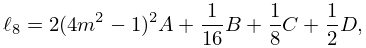
… ►and the coefficients ${\widetilde{𝒜}}_s(t)$ and ${\widetilde{ℬ}}_s(t)$ are given by … ►and the coefficients ${𝖠}_s(\tau )$ are the product of ${\tau }^s$ and a polynomial in $\tau$ of degree $2s$. …starting with ${𝖠}_0(\tau )=1$. … ►The coefficients $A_s(\zeta )$ and $B_s(\zeta )$ are given by …The coefficients $C_s(\zeta )$ and $D_s(\zeta )$ in (12.10.36) and (12.10.38) are given by …

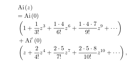
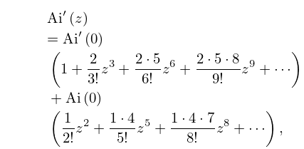
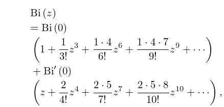
16: 9.4 Maclaurin Series

… ►

9.4.1 $$\mathrm{Ai}\left(z\right)=\mathrm{Ai}\left(0\right)\left(1+\frac{1}{3!}{z}^3+\frac{1\cdot 4}{6!}{z}^6+\frac{1\cdot 4\cdot 7}{9!}{z}^9+\mathrm{\cdots }\right)+{\mathrm{Ai}}^{\prime }\left(0\right)\left(z+\frac{2}{4!}{z}^4+\frac{2\cdot 5}{7!}{z}^7+\frac{2\cdot 5\cdot 8}{10!}{z}^{10}+\mathrm{\cdots }\right),$$

ⓘ

Symbols:

$\mathrm{Ai}\left(z\right)$: Airy function, $!$: factorial (as in $n!$) and $z$: complex variable

Source:

Olver (1997b, p. 54)

A&S Ref:

10.4.2 (with 10.4.4 and 10.4.5)

Permalink:

http://dlmf.nist.gov/9.4.E1

Encodings:

pMML, png, TeX

See also:

Annotations for §9.4 and Ch.9

►

9.4.2 $${\mathrm{Ai}}^{\prime }\left(z\right)={\mathrm{Ai}}^{\prime }\left(0\right)\left(1+\frac{2}{3!}{z}^3+\frac{2\cdot 5}{6!}{z}^6+\frac{2\cdot 5\cdot 8}{9!}{z}^9+\mathrm{\cdots }\right)+\mathrm{Ai}\left(0\right)\left(\frac{1}{2!}{z}^2+\frac{1\cdot 4}{5!}{z}^5+\frac{1\cdot 4\cdot 7}{8!}{z}^8+\mathrm{\cdots }\right),$$

ⓘ

Symbols:

$\mathrm{Ai}\left(z\right)$: Airy function, $!$: factorial (as in $n!$) and $z$: complex variable

Proof sketch:

Use methods of Olver (1997b, p. 54).

Permalink:

http://dlmf.nist.gov/9.4.E2

Encodings:

pMML, png, TeX

See also:

Annotations for §9.4 and Ch.9

►

9.4.3 $$\mathrm{Bi}\left(z\right)=\mathrm{Bi}\left(0\right)\left(1+\frac{1}{3!}{z}^3+\frac{1\cdot 4}{6!}{z}^6+\frac{1\cdot 4\cdot 7}{9!}{z}^9+\mathrm{\cdots }\right)+{\mathrm{Bi}}^{\prime }\left(0\right)\left(z+\frac{2}{4!}{z}^4+\frac{2\cdot 5}{7!}{z}^7+\frac{2\cdot 5\cdot 8}{10!}{z}^{10}+\mathrm{\cdots }\right),$$

ⓘ

Symbols:

$\mathrm{Bi}\left(z\right)$: Airy function, $!$: factorial (as in $n!$) and $z$: complex variable

Proof sketch:

Use methods of Olver (1997b, p. 54).

A&S Ref:

10.4.3 (with 10.4.4 and 10.4.5)

Referenced by:

(9.12.15)

Permalink:

http://dlmf.nist.gov/9.4.E3

Encodings:

pMML, png, TeX

See also:

Annotations for §9.4 and Ch.9

►

9.4.4 $${\mathrm{Bi}}^{\prime }\left(z\right)={\mathrm{Bi}}^{\prime }\left(0\right)\left(1+\frac{2}{3!}{z}^3+\frac{2\cdot 5}{6!}{z}^6+\frac{2\cdot 5\cdot 8}{9!}{z}^9+\mathrm{\cdots }\right)+\mathrm{Bi}\left(0\right)\left(\frac{1}{2!}{z}^2+\frac{1\cdot 4}{5!}{z}^5+\frac{1\cdot 4\cdot 7}{8!}{z}^8+\mathrm{\cdots }\right).$$

ⓘ

Symbols:

$\mathrm{Bi}\left(z\right)$: Airy function, $!$: factorial (as in $n!$) and $z$: complex variable

Proof sketch:

Use methods of Olver (1997b, p. 54).

Permalink:

http://dlmf.nist.gov/9.4.E4

Encodings:

pMML, png, TeX

See also:

Annotations for §9.4 and Ch.9

17: 24.2 Definitions and Generating Functions

… ►

Table 24.2.3: Bernoulli numbers $B_n=N/D$.

► ►►►

$n$	$N$	$D$	$B_n$
…
$8$	$-1$	$30$	$-\mathrm{3.33333\hspace{0.33em}3333}$	$\mathrm{\times 10⁻²}$
…

►

►

Table 24.2.4: Euler numbers $E_n$.

► ►►►

$n$	$E_n$
…
$8$	$1385$
…

►

►

Table 24.2.5: Coefficients $b_{n,k}$ of the Bernoulli polynomials $B_n\left(x\right)={\sum }_{k=0}^n{b}_{n,k}{x}^k$.

► ►►►

	$k$
$n$	$0$	$1$	$2$	$3$	$4$	$5$	$6$	$7$	$8$	$9$	$10$	$11$	$12$	$13$	$14$	$15$
…

►

►

Table 24.2.6: Coefficients $e_{n,k}$ of the Euler polynomials $E_n\left(x\right)={\sum }_{k=0}^n{e}_{n,k}{x}^k$.

► ►►►

	$k$
$n$	$0$	$1$	$2$	$3$	$4$	$5$	$6$	$7$	$8$	$9$	$10$	$11$	$12$	$13$	$14$	$15$
…

►

18: 34.14 Tables

§34.14 Tables

►Tables of exact values of the squares of the $\mathit{3}j$ and $\mathit{6}j$ symbols in which all parameters are $\le 8$ are given in Rotenberg et al. (1959), together with a bibliography of earlier tables of $\mathit{3}j,\mathit{6}j$, and $\mathit{9}j$ symbols on pp. … ►Some selected $\mathit{9}j$ symbols are also given. … 16-17; for $\mathit{9}j$ symbols on p. … ► 310–332, and for the $\mathit{9}j$ symbols on pp. …

19: 1.18 Linear Second Order Differential Operators and Eigenfunction Expansions

… ►Assume that $𝒟(T)$ is dense in $V$, i. … ► $u_{\lambda }\in 𝒟(T)$, corresponding to distinct eigenvalues, are orthogonal: i. … ►This insures the vanishing of the boundary terms in (1.18.26), and also is a choice which indicates that $𝒟(T)=𝒟(T^{\ast })$, as $f(x)$ and $g(x)$ satisfy the same boundary conditions and thus define the same domains. … ►More generally, continuous spectra may occur in sets of disjoint finite intervals $[{\lambda }_a,{\lambda }_b]\in (0,\mathrm{\infty })$, often called bands, when $q(x)$ is periodic, see Ashcroft and Mermin (1976, Ch 8) and Kittel (1996, Ch 7). … ►, $𝒟(T)\subset 𝒟(T^{\ast })$ and $T^{\ast }v=Tv$ for $v\in 𝒟(T)$. …

20: 19.37 Tables

… ►Tabulated for $\varphi =0(5^{\circ }){90}^{\circ }$, $k^2=0(.01)1$ to 10D by Fettis and Caslin (1964). ►Tabulated for $\varphi =0(1^{\circ }){90}^{\circ }$, $k^2=0(.01)1$ to 7S by Beli͡akov et al. (1962). … ►Tabulated for $\varphi =0(5^{\circ }){90}^{\circ }$, $k=0(.01)1$ to 10D by Fettis and Caslin (1964). ►Tabulated for $\varphi =0(5^{\circ }){90}^{\circ }$, $\arcsin k=0(1^{\circ }){90}^{\circ }$ to 6D by Byrd and Friedman (1971), for $\varphi =0(5^{\circ }){90}^{\circ }$, $\arcsin k=0(2^{\circ }){90}^{\circ }$ and $5^{\circ }({10}^{\circ }){85}^{\circ }$ to 8D by Abramowitz and Stegun (1964, Chapter 17), and for $\varphi =0({10}^{\circ }){90}^{\circ }$, $\arcsin k=0(5^{\circ }){90}^{\circ }$ to 9D by Zhang and Jin (1996, pp. 674–675). … ►Tabulated for $\varphi =5^{\circ }(5^{\circ }){80}^{\circ }({2.5}^{\circ }){90}^{\circ }$, ${\alpha }^2=-1(.1)-0.1,0.1(.1)1$, $k^2=0(.05)0.9(.02)1$ to 10D by Fettis and Caslin (1964) (and warns of inaccuracies in Selfridge and Maxfield (1958) and Paxton and Rollin (1959)). …