%E3%80%90%E4%BA%9A%E5%8D%9A%E4%BD%93%E8%82%B2qee9.com%E3%80%91%E6%9C%89%E9%87%91%E8%A7%92%E5%A4%A7%E7%8E%8B%E7%9A%84%E6%8D%95%E9%B1%BC%E6%B8%B8%E6%88%8F31jX

SearchAdvancedHelp

(0.027 seconds)

11—20 of 544 matching pages

11: 20.15 Tables

… ►This reference gives ${\theta }_j(x,q)$, $j=1,2,3,4$, and their logarithmic $x$-derivatives to 4D for $x/\pi =0(.1)1$, $\alpha =0(9^{\circ }){90}^{\circ }$, where $\alpha$ is the modular angle given by … ►Spenceley and Spenceley (1947) tabulates ${\theta }_1(x,q)/{\theta }_2(0,q)$, ${\theta }_2(x,q)/{\theta }_2(0,q)$, ${\theta }_3(x,q)/{\theta }_4(0,q)$, ${\theta }_4(x,q)/{\theta }_4(0,q)$ to 12D for $u=0(1^{\circ }){90}^{\circ }$, $\alpha =0(1^{\circ }){89}^{\circ }$, where $u=2x/(\pi {\theta }_3^2(0,q))$ and $\alpha$ is defined by (20.15.1), together with the corresponding values of ${\theta }_2(0,q)$ and ${\theta }_4(0,q)$. ►Lawden (1989, pp. 270–279) tabulates ${\theta }_j(x,q)$, $j=1,2,3,4$, to 5D for $x=0(1^{\circ }){90}^{\circ }$, $q=0.1(.1)0.9$, and also $q$ to 5D for $k^2=0(.01)1$. ►Tables of Neville’s theta functions ${\theta }_s(x,q)$, ${\theta }_c(x,q)$, ${\theta }_d(x,q)$, ${\theta }_n(x,q)$ (see §20.1) and their logarithmic $x$-derivatives are given in Abramowitz and Stegun (1964, pp. 582–585) to 9D for $\epsilon ,\alpha =0(5^{\circ }){90}^{\circ }$, where (in radian measure) $\epsilon =x/{\theta }_3^2(0,q)=\pi x/(2K\left(k\right))$, and $\alpha$ is defined by (20.15.1). …

12: 14.33 Tables

… ►

Abramowitz and Stegun (1964, Chapter 8) tabulates ${𝖯}_n\left(x\right)$ for $n=0(1)3,9,10$, $x=0(.01)1$, 5–8D; ${𝖯}_n^{\prime }\left(x\right)$ for $n=1(1)4,9,10$, $x=0(.01)1$, 5–7D; ${𝖰}_n\left(x\right)$ and ${𝖰}_n^{\prime }\left(x\right)$ for $n=0(1)3,9,10$, $x=0(.01)1$, 6–8D; $P_n\left(x\right)$ and $P_n^{\prime }\left(x\right)$ for $n=0(1)5,9,10$, $x=1(.2)10$, 6S; $Q_n\left(x\right)$ and $Q_n^{\prime }\left(x\right)$ for $n=0(1)3,9,10$, $x=1(.2)10$, 6S. (Here primes denote derivatives with respect to $x$.)

►

Zhang and Jin (1996, Chapter 4) tabulates ${𝖯}_n\left(x\right)$ for $n=2(1)5,10$, $x=0(.1)1$, 7D; ${𝖯}_n\left(\cos \theta \right)$ for $n=1(1)4,10$, $\theta =0(5^{\circ }){90}^{\circ }$, 8D; ${𝖰}_n\left(x\right)$ for $n=0(1)2,10$, $x=0(.1)0.9$, 8S; ${𝖰}_n\left(\cos \theta \right)$ for $n=0(1)3,10$, $\theta =0(5^{\circ }){90}^{\circ }$, 8D; ${𝖯}_n^m\left(x\right)$ for $m=1(1)4$, $n-m=0(1)2$, $n=10$, $x=0,0.5$, 8S; ${𝖰}_n^m\left(x\right)$ for $m=1(1)4$, $n=0(1)2,10$, 8S; ${𝖯}_{\nu }^m\left(\cos \theta \right)$ for $m=0(1)3$, $\nu =0(.25)5$, $\theta =0({15}^{\circ }){90}^{\circ }$, 5D; $P_n\left(x\right)$ for $n=2(1)5,10$, $x=1(1)10$, 7S; $Q_n\left(x\right)$ for $n=0(1)2,10$, $x=2(1)10$, 8S. Corresponding values of the derivative of each function are also included, as are 6D values of the first 5 $\nu$-zeros of ${𝖯}_{\nu }^m\left(\cos \theta \right)$ and of its derivative for $m=0(1)4$, $\theta ={10}^{\circ },{30}^{\circ },{150}^{\circ }$.

►

Belousov (1962) tabulates ${𝖯}_n^m\left(\cos \theta \right)$ (normalized) for $m=0(1)36$, $n-m=0(1)56$, $\theta =0({2.5}^{\circ }){90}^{\circ }$, 6D.

…

13: Bibliography K

… ►

A proof of the $q$-Macdonald-Morris conjecture for $B{C}_n$ . Mem. Amer. Math. Soc. 108 (516), pp. vi+80.

ⓘ

External Links:

ISSN 0065-9266, MathReview (Eric M. Opdam), ZentralBlatt

Referenced by:

§17.14.

Encodings:

BibTeX

… ►

Poly-Bernoulli numbers. J. Théor. Nombres Bordeaux 9 (1), pp. 221–228.

ⓘ

External Links:

ISSN 1246-7405, PostScript, MathReview (L. Skula), ZentralBlatt

Referenced by:

§24.16(iii).

Encodings:

BibTeX

… ►

Algorithm 763: INTERVAL_ARITHMETIC: A Fortran 90 module for an interval data type. ACM Trans. Math. Software 22 (4), pp. 385–392.

ⓘ

External Links:

ISSN 0098-3500, Document, GAMS (module 763; package TOMS), ZentralBlatt

Referenced by:

2nd item.

Encodings:

BibTeX

… ►

Nonsymmetric Askey-Wilson polynomials as vector-valued polynomials. Appl. Anal. 90 (3-4), pp. 731–746.

ⓘ

External Links:

ISSN 0003-6811, Link, MathReview (Masatoshi Iida), ZentralBlatt

Referenced by:

§18.38(iii), §18.38(iii).

Encodings:

BibTeX

… ►

On the zeros of the Fresnel integrals. Canad. J. Math. 9, pp. 118–131.

ⓘ

External Links:

MathReview (W. C. Rheinboldt), ZentralBlatt

Referenced by:

§7.13(iii).

Encodings:

BibTeX

…

14: 32.8 Rational Solutions

… ►

32.8.3 $$w(z;3)=\frac{3z^2}{z^3+4}-\frac{6z^2(z^3+10)}{z^6+20z^3-80},$$

ⓘ

Symbols:

$z$: real

Permalink:

http://dlmf.nist.gov/32.8.E3

Encodings:

pMML, png, TeX

See also:

Annotations for §32.8(ii), §32.8 and Ch.32

►

32.8.4 $$w(z;4)=-\frac{1}{z}+\frac{6z^2(z^3+10)}{z^6+20z^3-80}-\frac{9z^5(z^3+40)}{z^9+60z^6+11200}.$$

ⓘ

Symbols:

$z$: real

Permalink:

http://dlmf.nist.gov/32.8.E4

Encodings:

pMML, png, TeX

See also:

Annotations for §32.8(ii), §32.8 and Ch.32

… ►

$$Q_3(z)=z^6+20z^3-80,$$

… ►

$$Q_5(z)=z^{15}+140z^{12}+2800z^9+78400z^6-\mathrm{3\hspace{0.33em}13600}{z}^3-\mathrm{62\hspace{0.33em}72000},$$

… ►

$\alpha =\frac{1}{8}{(2m+1)}^2$, $\beta =-\frac{1}{8}{(2n+1)}^2$, and $\gamma \notin \mathbb{Z}$.

…

15: 5.16 Sums

… ►

5.16.1 $$\sum _{k=1}^{\mathrm{\infty }}{(-1)}^k{\psi }^{\prime }\left(k\right)=-\frac{{\pi }^2}{8},$$

ⓘ

Symbols:

$\pi$: the ratio of the circumference of a circle to its diameter, $\psi \left(z\right)$: psi (or digamma) function and $k$: nonnegative integer

Permalink:

http://dlmf.nist.gov/5.16.E1

Encodings:

pMML, png, TeX

See also:

Annotations for §5.16 and Ch.5

… ►For related sums involving finite field analogs of the gamma and beta functions (Gauss and Jacobi sums) see Andrews et al. (1999, Chapter 1) and Terras (1999, pp. 90, 149).

16: 26.13 Permutations: Cycle Notation

… ►

26.13.2

ⓘ

Referenced by:

§26.13, §26.13, §26.13

Permalink:

http://dlmf.nist.gov/26.13.E2

Encodings:

pMML, png, TeX

See also:

Annotations for §26.13 and Ch.26

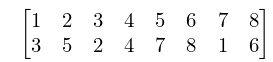
►is $\left(1,3,2,5,7\right)\left(4\right)\left(6,8\right)$ in cycle notation. …In consequence, (26.13.2) can also be written as $\left(1,3,2,5,7\right)\left(6,8\right)$. … ►For the example (26.13.2), this decomposition is given by $\left(1,3,2,5,7\right)\left(6,8\right)=\left(1,3\right)\left(2,3\right)\left(2,5\right)\left(5,7\right)\left(6,8\right).$ … ►Again, for the example (26.13.2) a minimal decomposition into adjacent transpositions is given by $\left(1,3,2,5,7\right)\left(6,8\right)=\left(2,3\right)\left(1,2\right)\left(4,5\right)\left(3,4\right)\left(2,3\right)\left(3,4\right)\left(4,5\right)\left(6,7\right)\left(5,6\right)\left(7,8\right)\left(6,7\right)$: $inv(\left(1,3,2,5,7\right)\left(6,8\right))=11$.

17: 1.11 Zeros of Polynomials

… ►Set $z=w-\frac{1}{3}a$ to reduce $f(z)=z^3+a{z}^2+bz+c$ to $g(w)=w^3+pw+q$, with $p=(3b-a^2)/3$, $q=(2a^3-9ab+27c)/27$. … ► $f(z)=z^3-6z^2+6z-2$, $g(w)=w^3-6w-6$, $A=3\sqrt[3]{4}$, $B=3\sqrt[3]{2}$. … ►Resolvent cubic is $z^3+12z^2+20z+9=0$ with roots ${\theta }_1=-1$, ${\theta }_2=-\frac{1}{2}(11+\sqrt{85})$, ${\theta }_3=-\frac{1}{2}(11-\sqrt{85})$, and $\sqrt{-{\theta }_1}=1$, $\sqrt{-{\theta }_2}=\frac{1}{2}(\sqrt{17}+\sqrt{5})$, $\sqrt{-{\theta }_3}=\frac{1}{2}(\sqrt{17}-\sqrt{5})$. … ►Let … ►Then $f(z)$, with $a_n\ne 0$, is stable iff $a_0\ne 0$; $D_{2k}>0$, $k=1,\mathrm{\dots },\lfloor \frac{1}{2}n\rfloor$; $\mathrm{sign}{D}_{2k+1}=\mathrm{sign}{a}_0$, $k=0,1,\mathrm{\dots },\lfloor \frac{1}{2}n-\frac{1}{2}\rfloor$.

18: 12.12 Integrals

… ►

12.12.2 $${\int }_0^{\mathrm{\infty }}{\mathrm{e}}^{-\frac{3}{4}{t}^2}{t}^{-a-\frac{3}{2}}U(a,t)dt=2^{\frac{1}{4}+\frac{1}{2}a}\mathrm{\Gamma }\left(-a-\frac{1}{2}\right)\cos \left((\frac{1}{4}a+\frac{1}{8})\pi \right),$$ ,

ⓘ

Symbols:

$\mathrm{\Gamma }\left(z\right)$: gamma function, $\pi$: the ratio of the circumference of a circle to its diameter, $\cos z$: cosine function, $dx$: differential of $x$ , $\mathrm{e}$: base of natural logarithm, $\int$: integral, $U(a,z)$: parabolic cylinder function, $\mathrm{\Re }$: real part and $a$: real or complex parameter

Permalink:

http://dlmf.nist.gov/12.12.E2

Encodings:

pMML, png, TeX

See also:

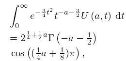
Annotations for §12.12 and Ch.12

… ►For compendia of integrals see Erdélyi et al. (1953b, v. 2, pp. 121–122), Erdélyi et al. (1954a, b, v. 1, pp. 60–61, 115, 210–211, and 336; v. 2, pp. 76–80, 115, 151, 171, and 395–398), Gradshteyn and Ryzhik (2000, §7.7), Magnus et al. (1966, pp. 330–331), Marichev (1983, pp. 190–191), Oberhettinger (1974, pp. 144–145), Oberhettinger (1990, pp. 106–108 and 192), Oberhettinger and Badii (1973, pp. 181–185), Prudnikov et al. (1986b, pp. 36–37, 155–168, 243–246, 289–290, 327–328, 419–420, and 619), Prudnikov et al. (1992a, §3.11), and Prudnikov et al. (1992b, §3.11). …

19: 10.34 Analytic Continuation

…

20: Bibliography J

… ►

Further results on the computation of incomplete gamma functions. In Analytic Theory of Continued Fractions, II (Pitlochry/Aviemore, 1985), W. J. Thron (Ed.), Lecture Notes in Math. 1199, pp. 67–89.

ⓘ

External Links:

MathReview (Marietta J. Tretter), ZentralBlatt

Referenced by:

§8.25(iv).

Encodings:

BibTeX

… ►

Density matrix of an impenetrable Bose gas and the fifth Painlevé transcendent. Phys. D 1 (1), pp. 80–158.

ⓘ

External Links:

ISSN 0167-2789, Document, MathReview, ZentralBlatt

Referenced by:

§32.16.

Encodings:

BibTeX

… ►

Modifications of Coulombic interactions by polarizable atoms. Math. Proc. Cambridge Philos. Soc. 80 (3), pp. 535–539.

ⓘ

External Links:

ISSN 0305-0041, Document, MathReview (Cataldo Agostinelli)

Referenced by:

§34.12.

Encodings:

BibTeX

… ►

Memoire sur l’itération des fonctions rationnelles. J. Math. Pures Appl. 8 (1), pp. 47–245 (French).

ⓘ

External Links:

FullText, ZentralBlatt

Referenced by:

§3.8(viii).

Encodings:

BibTeX