%E2%9A%BD%F0%9F%93%8F%20Koupit%20Ivermectin%20od%20%242.85%20%F0%9F%95%B5%20www.hPills.online%20%F0%9F%95%B5%20-%20Levn%C3%A9%20Pilulky%20%F0%9F%93%8F%E2%9A%BDM%C5%AF%C5%BEete%20Si%20Koupit%20Ivermectin%20V%20Mexiku%2C%20Kr%C3%A1tce%20Datovan%C3%BD%20Ivermectin%201%20Na%20Prodej%2C%20Koupit%20Ivermectin%20Kanada

SearchAdvancedHelp

(0.099 seconds)

21—30 of 853 matching pages

21: 1.1 Special Notation

… ► ►►►►►►

$x,y$	real variables.
…
${𝐀}^{-1}$	inverse of the square matrix $𝐀$
…
$det(𝐀)$	determinant of the square matrix $𝐀$
$\mathrm{tr}(𝐀)$	trace of the square matrix $𝐀$
$\mathrm{etr}\left(𝐀\right)$	exponential of $\mathrm{tr}(𝐀)$
…

►In the physics, applied maths, and engineering literature a common alternative to $\overline{a}$ is $a^{\ast }$, $a$ being a complex number or a matrix; the Hermitian conjugate of $𝐀$ is usually being denoted ${𝐀}^{†}$.

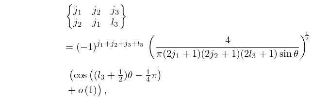
22: 34.8 Approximations for Large Parameters

§34.8 Approximations for Large Parameters

►For large values of the parameters in the $\mathit{3}j$, $\mathit{6}j$, and $\mathit{9}j$ symbols, different asymptotic forms are obtained depending on which parameters are large. … ►

34.8.1 $j_1,j_2,j_3\gg l_3\gg 1$,

ⓘ

Symbols:

$\pi$: the ratio of the circumference of a circle to its diameter, $\cos z$: cosine function, $o\left(x\right)$: order less than, $\sin z$: sine function, : $\mathit{6}j$ symbol, $j,j_r$: non-negative integers or non-negative integers plus one half. and $l,l_r$: non-negative integers or non-negative integers plus one half.

Permalink:

http://dlmf.nist.gov/34.8.E1

Encodings:

pMML, png, TeX

See also:

Annotations for §34.8 and Ch.34

… ►

34.8.2 $$\cos \theta =\frac{j_1(j_1+1)+j_2(j_2+1)-j_3(j_3+1)}{2\sqrt{j_1(j_1+1)j_2(j_2+1)}},$$

ⓘ

Symbols:

$\cos z$: cosine function and $j,j_r$: non-negative integers or non-negative integers plus one half.

Permalink:

http://dlmf.nist.gov/34.8.E2

Encodings:

pMML, png, TeX

See also:

Annotations for §34.8 and Ch.34

… ►For approximations for the $\mathit{3}j$, $\mathit{6}j$, and $\mathit{9}j$ symbols with error bounds see Flude (1998), Chen et al. (1999), and Watson (1999): these references also cite earlier work.

23: Bibliography

… ►

Evaluation of Coulomb wave functions along the transition line. Physical Rev. (2) 96, pp. 77–79.

ⓘ

External Links:

Document, MathReview (A. Erdélyi), ZentralBlatt

Referenced by:

§33.12(i).

Encodings:

BibTeX

… ►

Algorithm 610. A portable FORTRAN subroutine for derivatives of the psi function. ACM Trans. Math. Software 9 (4), pp. 494–502.

ⓘ

Notes:

Single and double precision, maximum accuracy 18S.

External Links:

ISSN 0098-3500, Document, GAMS (module 610; package TOMS), MathReview Entry, ZentralBlatt

Referenced by:

1st item.

Encodings:

BibTeX

… ►

Theorems on generalized Dedekind sums. Pacific J. Math. 2 (1), pp. 1–9.

ⓘ

External Links:

MathReview (N. G. de Bruijn), ZentralBlatt

Referenced by:

(25.11.41), (25.11.42), §25.11(xii).

Encodings:

BibTeX

… ►

Numerical Tables for Angular Correlation Computations in $\alpha$-, $\beta$- and $\gamma$-Spectroscopy: $3j$-, $6j$-, $9j$-Symbols, F- and $\mathrm{\Gamma }$-Coefficients. Landolt-Börnstein Numerical Data and Functional Relationships in Science and Technology, Springer-Verlag.

ⓘ

External Links:

ISBN 978-3-540-04218-1

Referenced by:

§34.14.

Encodings:

BibTeX

… ►

A new treatment of the ellipsoidal wave equation. Proc. London Math. Soc. (3) 9, pp. 21–50.

ⓘ

External Links:

ISSN 0024-6115, Document, MathReview (J. Meixner), ZentralBlatt

Referenced by:

§29.11.

Encodings:

BibTeX

…

24: 9.18 Tables

… ►

Miller (1946) tabulates $\mathrm{Ai}\left(x\right)$, ${\mathrm{Ai}}^{\prime }\left(x\right)$ for $x=-20(.01)2;$ ${\log }_{10}\mathrm{Ai}\left(x\right)$, ${\mathrm{Ai}}^{\prime }\left(x\right)/\mathrm{Ai}\left(x\right)$ for $x=0(.1)25(1)75$; $\mathrm{Bi}\left(x\right)$, ${\mathrm{Bi}}^{\prime }\left(x\right)$ for $x=-10(.1)2.5$; ${\log }_{10}\mathrm{Bi}\left(x\right)$, ${\mathrm{Bi}}^{\prime }\left(x\right)/\mathrm{Bi}\left(x\right)$ for $x=0(.1)10$; $M\left(x\right)$, $N\left(x\right)$, $\theta \left(x\right)$, $\varphi \left(x\right)$ (respectively $F(x)$, $G(x)$, $\chi (x)$, $\psi (x)$) for $x=-80(1)-30(.1)0$. Precision is generally 8D; slightly less for some of the auxiliary functions. Extracts from these tables are included in Abramowitz and Stegun (1964, Chapter 10), together with some auxiliary functions for large arguments.

… ►

Zhang and Jin (1996, p. 337) tabulates $\mathrm{Ai}\left(x\right)$, ${\mathrm{Ai}}^{\prime }\left(x\right)$, $\mathrm{Bi}\left(x\right)$, ${\mathrm{Bi}}^{\prime }\left(x\right)$ for $x=0(1)20$ to 8S and for $x=-20(1)0$ to 9D.

►

Yakovleva (1969) tabulates Fock’s functions $U(x)\equiv \sqrt{\pi }\mathrm{Bi}\left(x\right)$, $U^{\prime }(x)=\sqrt{\pi }{\mathrm{Bi}}^{\prime }\left(x\right)$, $V(x)\equiv \sqrt{\pi }\mathrm{Ai}\left(x\right)$, $V^{\prime }(x)=\sqrt{\pi }{\mathrm{Ai}}^{\prime }\left(x\right)$ for $x=-9(.001)9$. Precision is 7S.

… ►

National Bureau of Standards (1958) tabulates $A_0(x)\equiv \pi \mathrm{Hi}\left(-x\right)$ and $-A_0^{\prime }(x)\equiv \pi {\mathrm{Hi}}^{\prime }\left(-x\right)$ for $x=0(.01)1(.02)5(.05)11$ and $1/x=0.01(.01)0.1$; ${\int }_0^x{A}_0(t)dt$ for $x=0.5,1(1)11$. Precision is 8D.

►

Nosova and Tumarkin (1965) tabulates $e_0(x)\equiv \pi \mathrm{Hi}\left(-x\right)$, $e_0^{\prime }(x)=-\pi {\mathrm{Hi}}^{\prime }\left(-x\right)$, ${\tilde{e}}_0(-x)\equiv -\pi \mathrm{Gi}\left(x\right)$, ${\tilde{e}}_0^{\prime }(-x)=\pi {\mathrm{Gi}}^{\prime }\left(x\right)$ for $x=-1(.01)10$; 7D. Also included are the real and imaginary parts of $e_0(z)$ and $\mathrm{i}{e}_0^{\prime }(z)$, where $z=\mathrm{i}y$ and $y=0(.01)9$; 6-7D.

…

25: 11.11 Asymptotic Expansions of Anger–Weber Functions

… ►Let $F_0(\nu )=G_0(\nu )=1$, and for $k=1,2,3,\mathrm{\dots }$, … ►

$a_2(\lambda )={\displaystyle \frac{9{\lambda }^2-\lambda }{24{(1+\lambda )}^7}},$

… ►Also, as $\nu \to \mathrm{\infty }$ in $|\mathrm{ph}\nu |\le 2\pi -\delta$, … ►When $\nu$ is real and positive, all of (11.11.10)–(11.11.17) can be regarded as special cases of two asymptotic expansions given in Olver (1997b, pp. 352–360) for ${𝐀}_{-\nu }\left(\lambda \nu \right)$ as $\nu \to +\mathrm{\infty }$, one being uniform for , and the other being uniform for $\lambda \ge 1$. (Note that Olver’s definition of ${𝐀}_{\nu }\left(z\right)$ omits the factor $1/\pi$ in (11.10.4).) …

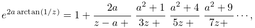
26: 4.25 Continued Fractions

… ►

4.25.2 $$\tan \left(az\right)=\frac{a\tan z}{1+}\frac{(1-a^2){\tan }^{2}z}{3+}\frac{(4-a^2){\tan }^{2}z}{5+}\frac{(9-a^2){\tan }^{2}z}{7+}\mathrm{\cdots },$$ , $az\ne \pm \frac{1}{2}\pi ,\pm \frac{3}{2}\pi ,\mathrm{\dots }$.

ⓘ

Symbols:

$\pi$: the ratio of the circumference of a circle to its diameter, $\mathrm{\Re }$: real part, $\tan z$: tangent function, $a$: real or complex constant and $z$: complex variable

A&S Ref:

4.3.95

Permalink:

http://dlmf.nist.gov/4.25.E2

Encodings:

pMML, png, TeX

See also:

Annotations for §4.25 and Ch.4

►

4.25.3 $$\frac{\arcsin z}{\sqrt{1-z^2}}=\frac{z}{1-}\frac{1\cdot 2z^2}{3-}\frac{1\cdot 2z^2}{5-}\frac{3\cdot 4z^2}{7-}\frac{3\cdot 4z^2}{9-}\mathrm{\cdots },$$

ⓘ

Symbols:

$\arcsin z$: arcsine function and $z$: complex variable

A&S Ref:

4.4.44

Permalink:

http://dlmf.nist.gov/4.25.E3

Encodings:

pMML, png, TeX

See also:

Annotations for §4.25 and Ch.4

… ►

4.25.4 $$\arctan z=\frac{z}{1+}\frac{z^2}{3+}\frac{4z^2}{5+}\frac{9z^2}{7+}\frac{16z^2}{9+}\mathrm{\cdots },$$

ⓘ

Symbols:

$\arctan z$: arctangent function and $z$: complex variable

A&S Ref:

4.4.43

Referenced by:

§3.10(ii)

Permalink:

http://dlmf.nist.gov/4.25.E4

Encodings:

pMML, png, TeX

See also:

Annotations for §4.25 and Ch.4

… ►

4.25.5 $${\mathrm{e}}^{2a\arctan \left(1/z\right)}=1+\frac{2a}{z-a+}\frac{a^2+1}{3z+}\frac{a^2+4}{5z+}\frac{a^2+9}{7z+}\mathrm{\cdots },$$

ⓘ

Symbols:

$\mathrm{e}$: base of natural logarithm, $\arctan z$: arctangent function, $a$: real or complex constant and $z$: complex variable

A&S Ref:

4.2.42

Permalink:

http://dlmf.nist.gov/4.25.E5

Encodings:

pMML, png, TeX

See also:

Annotations for §4.25 and Ch.4

… ►See also Cuyt et al. (2008, pp. 201–203, 205–210).

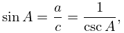
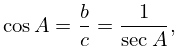
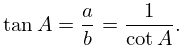
27: 4.42 Solution of Triangles

… ►

4.42.1 $$\sin A=\frac{a}{c}=\frac{1}{\csc A},$$

ⓘ

Symbols:

$\csc z$: cosecant function, $\sin z$: sine function, $A$: angle, $a$: height and $c$: hypotenuse

A&S Ref:

4.3.147

Permalink:

http://dlmf.nist.gov/4.42.E1

Encodings:

pMML, png, TeX

See also:

Annotations for §4.42(i), §4.42 and Ch.4

►

4.42.2 $$\cos A=\frac{b}{c}=\frac{1}{\sec A},$$

ⓘ

Symbols:

$\cos z$: cosine function, $\sec z$: secant function, $A$: angle, $b$: base and $c$: hypotenuse

A&S Ref:

4.3.147

Permalink:

http://dlmf.nist.gov/4.42.E2

Encodings:

pMML, png, TeX

See also:

Annotations for §4.42(i), §4.42 and Ch.4

►

4.42.3 $$\tan A=\frac{a}{b}=\frac{1}{\cot A}.$$

ⓘ

Symbols:

$\cot z$: cotangent function, $\tan z$: tangent function, $A$: angle, $a$: height and $b$: base

A&S Ref:

4.3.147

Permalink:

http://dlmf.nist.gov/4.42.E3

Encodings:

pMML, png, TeX

See also:

Annotations for §4.42(i), §4.42 and Ch.4

… ►

4.42.7 $$\text{area}=\frac{1}{2}bc\sin A={\left(s(s-a)(s-b)(s-c)\right)}^{1/2},$$

ⓘ

Symbols:

$\sin z$: sine function, $a$: length, $b$: base, $c$: length, $s$: semi-perimeter and $A$: angle

A&S Ref:

4.3.148

Permalink:

http://dlmf.nist.gov/4.42.E7

Encodings:

pMML, png, TeX

See also:

Annotations for §4.42(ii), §4.42 and Ch.4

►where $s=\frac{1}{2}(a+b+c)$ (the semiperimeter). …

28: 1.11 Zeros of Polynomials

… ►where $z_1,z_2,\mathrm{\dots },z_n$ are the zeros of $f(z)$. … ►The roots of $a{z}^2+bz+c=0$ are … ►Set $z=w-\frac{1}{3}a$ to reduce $f(z)=z^3+a{z}^2+bz+c$ to $g(w)=w^3+pw+q$, with $p=(3b-a^2)/3$, $q=(2a^3-9ab+27c)/27$. … ► $f(z)=z^3-6z^2+6z-2$, $g(w)=w^3-6w-6$, $A=3\sqrt[3]{4}$, $B=3\sqrt[3]{2}$. … ►Resolvent cubic is $z^3+12z^2+20z+9=0$ with roots ${\theta }_1=-1$, ${\theta }_2=-\frac{1}{2}(11+\sqrt{85})$, ${\theta }_3=-\frac{1}{2}(11-\sqrt{85})$, and $\sqrt{-{\theta }_1}=1$, $\sqrt{-{\theta }_2}=\frac{1}{2}(\sqrt{17}+\sqrt{5})$, $\sqrt{-{\theta }_3}=\frac{1}{2}(\sqrt{17}-\sqrt{5})$. …

29: 10.41 Asymptotic Expansions for Large Order

… ►Also, $U_k(p)$ and $V_k(p)$ are polynomials in $p$ of degree $3k$, given by $U_0(p)=V_0(p)=1$, and … ►For $k=1,2,3$, … ►For numerical tables of $\eta =\eta (z)$ and the coefficients $U_k(p)$, $V_k(p)$, see Olver (1962, pp. 43–51). … ►The expansions (10.41.3)–(10.41.6) also hold uniformly in the sector $|\mathrm{ph}z|\le \frac{1}{2}\pi -\delta$ , with the branches of the fractional powers in (10.41.3)–(10.41.8) extended by continuity from the positive real $z$-axis. … ►This is because $A_k(\zeta )$ and ${\zeta }^{-\frac{1}{2}}{B}_k(\zeta ),k=0,1,\mathrm{\dots }$, do not form an asymptotic scale (§2.1(v)) as $\zeta \to +\mathrm{\infty }$; see Olver (1997b, pp. 422–425). …

30: 18.8 Differential Equations

… ►

Table 18.8.1: Classical OP’s: differential equations $A(x)f^{\prime \prime }(x)+B(x)f^{\prime }(x)+C(x)f(x)+{\lambda }_{n}f(x)=0$.

► ►►►►►

#	$f(x)$	$A(x)$	$B(x)$	$C(x)$	${\lambda }_n$
1	$P_n^{(\alpha ,\beta )}\left(x\right)$	$1-x^2$	$\beta -\alpha -(\alpha +\beta +2)x$	0	$n(n+\alpha +\beta +1)$
…
8	$L_n^{(\alpha )}\left(x\right)$	$x$	$\alpha +1-x$	$0$	$n$
9	${\mathrm{e}}^{-\frac{1}{2}{x}^2}{x}^{\alpha +\frac{1}{2}}{L}_n^{(\alpha )}\left(x^2\right)$	$1$	$0$	$-x^2+(\frac{1}{4}-{\alpha }^2)x^{-2}$	$4n+2\alpha +2$
…

►

…