values at z=0

SearchAdvancedHelp

(0.005 seconds)

41—50 of 144 matching pages

41: 1.9 Calculus of a Complex Variable

… ►A function $f(z)$ is continuous at a point $z_0$ if $\underset{z\to z_0}{lim}f(z)=f(z_0)$. … ►A function of two complex variables $f(z,w)$ is continuous at $(z_0,w_0)$ if $\underset{(z,w)\to (z_0,w_0)}{lim}f(z,w)=f(z_0,w_0)$; compare (1.5.1) and (1.5.2). … ►A function $f(z)$ is said to be analytic (holomorphic) at $z=z_0$ if it is complex differentiable in a neighborhood of $z_0$. … ►A function $f(z)$ is analytic at $\mathrm{\infty }$ if $g(z)=f(1/z)$ is analytic at $z=0$, and we set $f^{\prime }(\mathrm{\infty })=g^{\prime }(0)$. … ►We then say that the mapping $w=f(z)$ is conformal (angle-preserving) at $z_0$. …

42: 10.20 Uniform Asymptotic Expansions for Large Order

… ►that is infinitely differentiable on the interval , including $z=1$. …all functions taking their principal values, with $\zeta =\mathrm{\infty },0,-\mathrm{\infty }$, corresponding to $z=0,1,\mathrm{\infty }$, respectively. … ►

Interval

… ►

Values at $\zeta =0$

… ►As $\nu \to \mathrm{\infty }$ through positive real values the expansions (10.20.4)–(10.20.9) apply uniformly for $|\mathrm{ph}z|\le \pi -\delta$, the coefficients $A_k(\zeta )$, $B_k(\zeta )$, $C_k(\zeta )$, and $D_k(\zeta )$, being the analytic continuations of the functions defined in §10.20(i) when $\zeta$ is real. …

43: 5.2 Definitions

… ►When $\mathrm{\Re }z\le 0$, $\mathrm{\Gamma }\left(z\right)$ is defined by analytic continuation. It is a meromorphic function with no zeros, and with simple poles of residue ${(-1)}^n/n!$ at $z=-n$. $1/\mathrm{\Gamma }\left(z\right)$ is entire, with simple zeros at $z=-n$. …$\psi \left(z\right)$ is meromorphic with simple poles of residue $-1$ at $z=-n$. … ►in which $L(n,k)=\left(\genfrac{}{}{0.0pt}{}{n-1}{k-1}\right)\frac{n!}{k!}$ is the Lah number. …

44: 25.12 Polylogarithms

… ►Other notations and names for ${\mathrm{Li}}_2\left(z\right)$ include $S_2(z)$ (Kölbig et al. (1970)), Spence function $\mathrm{Sp}(z)$ (’t Hooft and Veltman (1979)), and ${\mathrm{L}}_2(z)$ (Maximon (2003)). ►In the complex plane ${\mathrm{Li}}_2\left(z\right)$ has a branch point at $z=1$. … ►When $z={\mathrm{e}}^{\mathrm{i}\theta }$, $0\le \theta \le 2\pi$, (25.12.1) becomes … ►For other values of $z$, ${\mathrm{Li}}_s\left(z\right)$ is defined by analytic continuation. … ►valid when $\mathrm{\Re }s>0$ and , or $\mathrm{\Re }s>1$ and $z=1$. …

45: 11.10 Anger–Weber Functions

… ►The Anger function ${𝐉}_{\nu }\left(z\right)$ and Weber function ${𝐄}_{\nu }\left(z\right)$ are defined by …Each is an entire function of $z$ and $\nu$. … ►(11.10.4) also applies when $\mathrm{\Re }z=0$ and $\mathrm{\Re }\nu >0$. … ►These expansions converge absolutely for all finite values of $z$. … ►

§11.10(vii) Special Values

…

46: 10.3 Graphics

… ►In the graphics shown in this subsection, height corresponds to the absolute value of the function and color to the phase. … ►

►

►

Figure 10.3.10: $H_0^{(1)}\left(x+\mathrm{i}y\right)$, $-10\le x\le 5$, $-2.8\le y\le 4$. Principal value. … Magnify 3D Help

… ►

►

►

Figure 10.3.12: $H_1^{(1)}\left(x+\mathrm{i}y\right)$, $-10\le x\le 5$, $-2.8\le y\le 4$. Principal value. … Magnify 3D Help

… ►

►

►

Figure 10.3.14: $H_5^{(1)}\left(x+\mathrm{i}y\right)$, $-20\le x\le 10$, $-4\le y\le 4$. Principal value. … Magnify 3D Help

►

►

►

Figure 10.3.15: $J_{5.5}\left(x+\mathrm{i}y\right)$, $-10\le x\le 10$, $-4\le y\le 4$. Principal value. … Magnify 3D Help

…

47: 5.9 Integral Representations

… ► $\mathrm{\Re }\nu >0$, $\mu >0$, and $\mathrm{\Re }z>0$. (The fractional powers have their principal values.) … ► $t^{-z}$ has its principal value where $t$ crosses the positive real axis, and is continuous. … ►where and the inverse tangent has its principal value. … ►For $\mathrm{\Re }z>0$, …

48: 22.20 Methods of Computation

… ►A powerful way of computing the twelve Jacobian elliptic functions for real or complex values of both the argument $z$ and the modulus $k$ is to use the definitions in terms of theta functions given in §22.2, obtaining the theta functions via methods described in §20.14. … ►For $x$ real and $k\in (0,1)$, use (22.20.1) with $a_0=1$, $b_0=k^{\prime }\in (0,1)$, $c_0=k$, and continue until $c_N$ is zero to the required accuracy. …and the inverse sine has its principal value (§4.23(ii)). …If only the value of $\mathrm{dn}(x,k)$ at $x=K$ is required then the exact value is in the table 22.5.1. … ►If either $\tau$ or $q={\mathrm{e}}^{\mathrm{i}\pi \tau }$ is given, then we use $k={\theta }_2^2(0,q)/{\theta }_3^2(0,q)$, $k^{\prime }={\theta }_4^2(0,q)/{\theta }_3^2(0,q)$, $K=\frac{1}{2}\pi {\theta }_3^2(0,q)$, and $K^{\prime }=-\mathrm{i}\tau K$, obtaining the values of the theta functions as in §20.14. …

49: 8.19 Generalized Exponential Integral

… ►When the path of integration excludes the origin and does not cross the negative real axis (8.19.2) defines the principal value of $E_p\left(z\right)$, and unless indicated otherwise in the DLMF principal values are assumed. … ►

§8.19(iii) Special Values

… ►Unless $p$ is a nonpositive integer, $E_p\left(z\right)$ has a branch point at $z=0$. For $z\ne 0$ each branch of $E_p\left(z\right)$ is an entire function of $p$. … ►For $n=1,2,3,\mathrm{\dots }$ and $x>0$, …

50: 19.17 Graphics

… ►Because the $R$-function is homogeneous, there is no loss of generality in giving one variable the value $1$ or $-1$ (as in Figure 19.3.2). For $R_F$, $R_G$, and $R_J$, which are symmetric in $x,y,z$, we may further assume that $z$ is the largest of $x,y,z$ if the variables are real, then choose $z=1$, and consider only $0\le x\le 1$ and $0\le y\le 1$. The cases $x=0$ or $y=0$ correspond to the complete integrals. 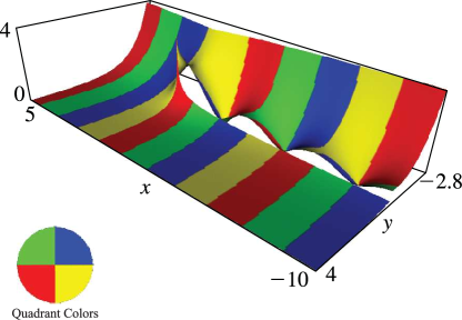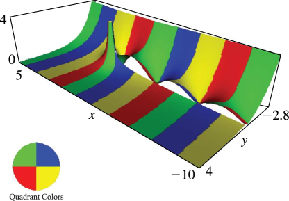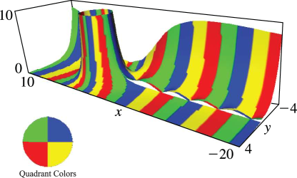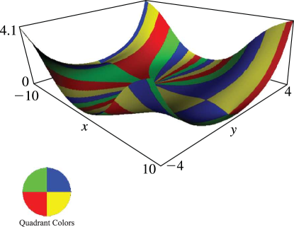… ►To view $R_F(0,y,1)$ and $2R_G(0,y,1)$ for complex $y$, put $y=1-k^2$, use (19.25.1), and see Figures 19.3.7–19.3.12. … ►To view $R_F(0,y,1)$ and $2R_G(0,y,1)$ for complex $y$, put $y=1-k^2$, use (19.25.1), and see Figures 19.3.7–19.3.12. …