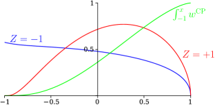
About the Project

discrete weights

AdvancedHelp

(0.001 seconds)

1—10 of 14 matching pages

1: 18.39 Applications in the Physical Sciences
See accompanying text
Figure 18.39.2: Coulomb–Pollaczek weight functions, x [ 1 , 1 ] , (18.39.50) for s = 10 , l = 0 , and Z = ± 1 . …For Z = 1 the weight function, blue curve, is non-zero at x = 1 , but this point is also an essential singularity as the discrete parts of the weight function of (18.39.51) accumulate as k , x k 1 . Magnify
In the attractive case (18.35.6_4) for the discrete parts of the weight function where with x k < 1 , are also simplified: …
w x k CP = ( l + 1 + 2 Z s ) ρ 2 k 1 ( 1 ρ 2 ) 2 l + 3 ( 2 l + 2 ) k 2 ( k + l + 1 ) k ! .
2: 18.30 Associated OP’s
For other cases there may also be, in addition to a possible integral as in (18.30.10), a finite sum of discrete weights on the negative real x -axis each multiplied by the polynomial product evaluated at the corresponding values of x , as in (18.2.3). …
3: 18.19 Hahn Class: Definitions
Table 18.19.1: Orthogonality properties for Hahn, Krawtchouk, Meixner, and Charlier OP’s: discrete sets, weight functions, standardizations, and parameter constraints.
p n ( x ) X w x h n
4: 18.28 Askey–Wilson Class
The Askey–Wilson polynomials form a system of OP’s { p n ( x ) } , n = 0 , 1 , 2 , , that are orthogonal with respect to a weight function on a bounded interval, possibly supplemented with discrete weights on a finite set. …
5: 18.25 Wilson Class: Definitions
§18.25(iii) Weights and Normalizations: Discrete Cases
6: 18.38 Mathematical Applications
The basic ideas of Gaussian quadrature, and their extensions to non-classical weight functions, and the computation of the corresponding quadrature abscissas and weights, have led to discrete variable representations, or DVRs, of Sturm–Liouville and other differential operators. …
7: 3.11 Approximation Techniques
Now suppose that X k = 0 when k , that is, the functions ϕ k ( x ) are orthogonal with respect to weighted summation on the discrete set x 1 , x 2 , , x J . …
8: 18.35 Pollaczek Polynomials
where, depending on a , b , λ , D is a discrete subset of and the w ζ ( λ ) ( a , b ) are certain weights. …
9: 18.3 Definitions
Table 18.3.1: Orthogonality properties for classical OP’s: intervals, weight functions, standardizations, leading coefficients, and parameter constraints. …
Name p n ( x ) ( a , b ) w ( x ) h n k n k ~ n / k n Constraints
In addition to the orthogonal property given by Table 18.3.1, the Chebyshev polynomials T n ( x ) , n = 0 , 1 , , N , are orthogonal on the discrete point set comprising the zeros x N + 1 , n , n = 1 , 2 , , N + 1 , of T N + 1 ( x ) : … For another version of the discrete orthogonality property of the polynomials T n ( x ) see (3.11.9). … It is also related to a discrete Fourier-cosine transform, see Britanak et al. (2007). … For 1 β > α > 1 a finite system of Jacobi polynomials P n ( α , β ) ( x ) is orthogonal on ( 1 , ) with weight function w ( x ) = ( x 1 ) α ( x + 1 ) β . …
10: Bibliography Z
  • D. Zeilberger and D. M. Bressoud (1985) A proof of Andrews’ q -Dyson conjecture. Discrete Math. 54 (2), pp. 201–224.
  • J. Zeng (1992) Weighted derangements and the linearization coefficients of orthogonal Sheffer polynomials. Proc. London Math. Soc. (3) 65 (1), pp. 1–22.