.2022世界杯中国男足蠃_『welcom_』世界杯冠军加多少分_w2n3c1o_2022年12月10日16时49分8秒_zwuzf2w8s

SearchAdvancedHelp

(0.004 seconds)

11—20 of 355 matching pages

11: 26.21 Tables

… ►Abramowitz and Stegun (1964, Chapter 24) tabulates binomial coefficients $\left(\genfrac{}{}{0.0pt}{}{m}{n}\right)$ for $m$ up to 50 and $n$ up to 25; extends Table 26.4.1 to $n=10$; tabulates Stirling numbers of the first and second kinds, $s(n,k)$ and $S(n,k)$, for $n$ up to 25 and $k$ up to $n$; tabulates partitions $p\left(n\right)$ and partitions into distinct parts $p(𝒟,n)$ for $n$ up to 500. … ►It also contains a table of Gaussian polynomials up to ${\left[\genfrac{}{}{0.0pt}{}{12}{6}\right]}_q$. …

12: 18.41 Tables

… ►Abramowitz and Stegun (1964, Tables 22.4, 22.6, 22.11, and 22.13) tabulates $T_n\left(x\right)$, $U_n\left(x\right)$, $L_n\left(x\right)$, and $H_n\left(x\right)$ for $n=0(1)12$. The ranges of $x$ are $0.2(.2)1$ for $T_n\left(x\right)$ and $U_n\left(x\right)$, and $0.5,1,3,5,10$ for $L_n\left(x\right)$ and $H_n\left(x\right)$. …

13: 30.7 Graphics

… ►

►►

Figure 30.7.1: Eigenvalues ${\lambda }_n^0\left({\gamma }^2\right)$, $n=0,1,2,3$, $-10\le {\gamma }^2\le 10$. Magnify

►

►►

Figure 30.7.2: Eigenvalues ${\lambda }_n^1\left({\gamma }^2\right)$ $n=1,2,3,4$, $-10\le {\gamma }^2\le 10$. Magnify

►

►►

Figure 30.7.3: Eigenvalues ${\lambda }_n^5\left({\gamma }^2\right)$, $n=5,6,7,8$, $-40\le {\gamma }^2\le 40$. Magnify

►

►►

Figure 30.7.4: Eigenvalues ${\lambda }_n^{10}\left({\gamma }^2\right)$, $n=10,11,12,13$, $-50\le {\gamma }^2\le 150$. Magnify

… ►

►

►

Figure 30.7.15: . Magnify 3D Help

…

14: 26.10 Integer Partitions: Other Restrictions

… ►

Table 26.10.1: Partitions restricted by difference conditions, or equivalently with parts from $A_{j,k}$.

► ►►►►►►►

	$p(𝒟,n)$	$p(𝒟2,n)$	$p(𝒟2,\in T,n)$	$p({𝒟}^{\prime }3,n)$
…
$10$	$10$	$6$	$4$	$4$
$11$	$12$	$7$	$4$	$5$
$12$	$15$	$9$	$6$	$6$
…
$14$	$22$	$12$	$8$	$8$
…
$17$	$38$	$19$	$12$	$12$
…

►

…

15: 25.3 Graphics

… ►

►►

Figure 25.3.1: Riemann zeta function $\zeta \left(x\right)$ and its derivative ${\zeta }^{\prime }\left(x\right)$, $-20\le x\le 10$. Magnify

►

►►

Figure 25.3.2: Riemann zeta function $\zeta \left(x\right)$ and its derivative ${\zeta }^{\prime }\left(x\right)$, $-12\le x\le -2$. Magnify

►

►

►

Figure 25.3.3: Modulus of the Riemann zeta function $|\zeta \left(x+\mathrm{i}y\right)|$, $-4\le x\le 4$, $-10\le y\le 40$. Magnify 3D Help

…

16: 26.9 Integer Partitions: Restricted Number and Part Size

… ►

Table 26.9.1: Partitions $p_k\left(n\right)$.

► ►►►►►►

$n$	$k$
	0	1	2	3	4	5	6	7	8	9	10
…
6	0	1	4	7	9	10	11	11	11	11	11
…
8	0	1	5	10	15	18	20	21	22	22	22
9	0	1	5	12	18	23	26	28	29	30	30
…

►

… ►

$p_3\left(n\right)=1+\lfloor {\displaystyle \frac{n^2+6n}{12}}\rfloor .$

…

17: 10.48 Graphs

… ►

►►

Figure 10.48.1: ${𝗃}_n\left(x\right)$, $n=0(1)4$, $0\le x\le 12$. Magnify

►

►►

Figure 10.48.2: ${𝗒}_n\left(x\right)$, $n=0(1)4$, . Magnify

►

►►

Figure 10.48.3: ${𝗃}_5\left(x\right)$, ${𝗒}_5\left(x\right)$, $\sqrt{{𝗃}_5^2\left(x\right)+{𝗒}_5^2\left(x\right)}$, $0\le x\le 12$. Magnify

►

►►

Figure 10.48.4: ${𝗃}_5^{\prime }\left(x\right)$, ${𝗒}_5^{\prime }\left(x\right)$, $\sqrt{𝗃_5^{\prime }{}_{}{}^2\left(x\right)+𝗒_5^{\prime }{}_{}{}^2\left(x\right)}$, $0\le x\le 12$. Magnify

… ►

►►

Figure 10.48.7: ${𝗂}_5^{(1)}\left(x\right)$, ${𝗂}_5^{(2)}\left(x\right)$, ${𝗄}_5\left(x\right)$, $0\le x\le 8$. Magnify

18: 11.14 Tables

… ►

Abramowitz and Stegun (1964, Chapter 12) tabulates ${𝐇}_n\left(x\right)$, ${𝐇}_n\left(x\right)-Y_n\left(x\right)$, and $I_n\left(x\right)-{𝐋}_n\left(x\right)$ for $n=0,1$ and $x=0(.1)5$, $x^{-1}=0(.01)0.2$ to 6D or 7D.

… ►

Barrett (1964) tabulates ${𝐋}_n\left(x\right)$ for $n=0,1$ and $x=0.2(.005)4(.05)10(.1)19.2$ to 5 or 6S, $x=6(.25)59.5(.5)100$ to 2S.

… ►

Abramowitz and Stegun (1964, Chapter 12) tabulates ${\int }_0^x(I_0\left(t\right)-{𝐋}_0\left(t\right))dt$ and $(2/\pi ){\int }_x^{\mathrm{\infty }}{t}^{-1}{𝐇}_0\left(t\right)dt$ for $x=0(.1)5$ to 5D or 7D; ${\int }_0^x({𝐇}_0\left(t\right)-Y_0\left(t\right))dt-(2/\pi )\ln x$, ${\int }_0^x(I_0\left(t\right)-{𝐋}_0\left(t\right))dt-(2/\pi )\ln x$, and ${\int }_x^{\mathrm{\infty }}{t}^{-1}({𝐇}_0\left(t\right)-Y_0\left(t\right))dt$ for $x^{-1}=0(.01)0.2$ to 6D.

… ►

Bernard and Ishimaru (1962) tabulates ${𝐉}_{\nu }\left(x\right)$ and ${𝐄}_{\nu }\left(x\right)$ for $\nu =-10(.1)10$ and $x=0(.1)10$ to 5D.

… ►

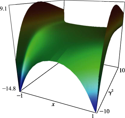
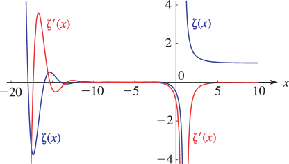
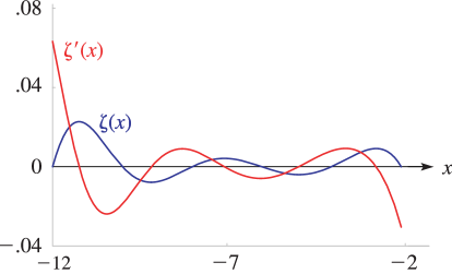
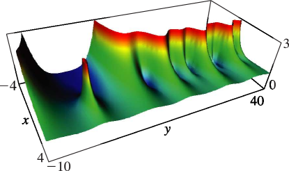
Agrest and Maksimov (1971, Chapter 11) defines incomplete Struve, Anger, and Weber functions and includes tables of an incomplete Struve function ${𝐇}_n\left(x,\alpha \right)$ for $n=0,1$, $x=0(.2)10$, and $\alpha =0(.2)1.4,\frac{1}{2}\pi$, together with surface plots.

19: 26.2 Basic Definitions

… ►

Table 26.2.1: Partitions $p\left(n\right)$.

► ►►►►►

$n$	$p\left(n\right)$	$n$	$p\left(n\right)$	$n$	$p\left(n\right)$
…
8	22	25	1958	42	53174
…
10	42	27	3010	44	75175
…
12	77	29	4565	46	1 05558
…

►

20: Publications

… ►

The NIST Digital Library of Mathematical Functions Project, Annals of Mathematics and Artificial Intelligence—Special Issue on Mathematical Knowledge Management, Vol. 38, Nos. 1–3, pp. 105–119.

… ►

Boundary/Contour Fitted Grid Generation for Effective Visualizations in a Digital Library of Mathematical Functions, Proceedings of the 9th International Conference on Numerical Grid Generation in Computational Field Simulations, San Jose, June 11–18, 2005. pp. 61–71.

… ►

From B-Spline Mesh Generation to Effective Visualizations for the NIST Digital Library of Mathematical Functions, in Curve and Surface Design, Proceedings of the Sixth International Conference on Curves and Surfaces, Avignon, France June 29–July 5, 2006, pp. 235–243.

…
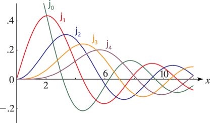
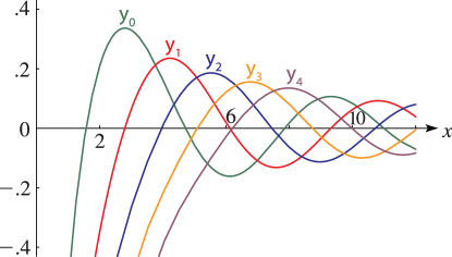
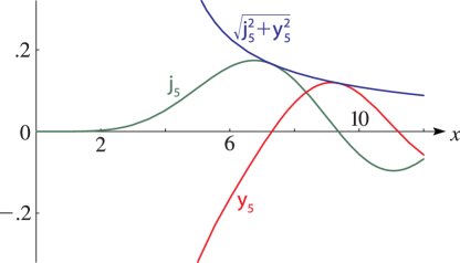
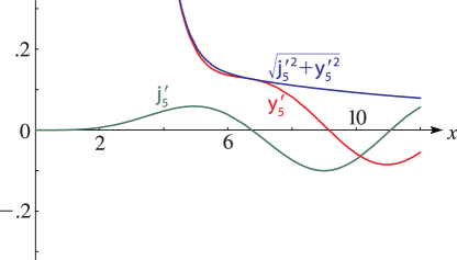