§30.13 Wave Equation in Prolate Spheroidal Coordinates
Contents
- §30.13(i) Prolate Spheroidal Coordinates
- §30.13(ii) Metric Coefficients
- §30.13(iii) Laplacian
- §30.13(iv) Separation of Variables
- §30.13(v) The Interior Dirichlet Problem for Prolate Ellipsoids
§30.13(i) Prolate Spheroidal Coordinates
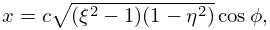
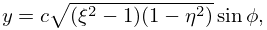
Prolate spheroidal coordinates are related to Cartesian coordinates by
| 30.13.1 | ||||
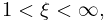
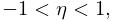
where is a positive constant. (On the use of the symbol in place of see §1.5(ii).) The -space without the -axis corresponds to
| 30.13.2 | ||||
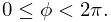
The coordinate surfaces are prolate ellipsoids of revolution with foci at , . The coordinate surfaces are sheets of two-sheeted hyperboloids of revolution with the same foci. The focal line is given by , , and the rays , are given by , .
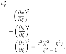
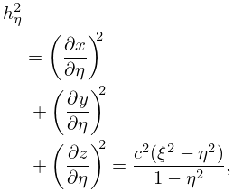
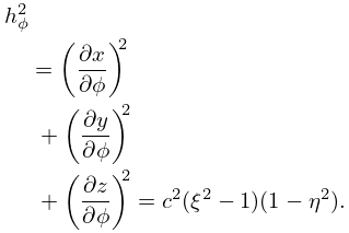
§30.13(ii) Metric Coefficients
| 30.13.3 | ||||
| 30.13.4 | ||||
| 30.13.5 | ||||
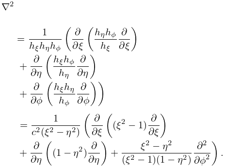
§30.13(iii) Laplacian
| 30.13.6 | |||
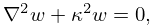
§30.13(iv) Separation of Variables
The wave equation
| 30.13.7 | |||
transformed to prolate spheroidal coordinates , admits solutions
| 30.13.8 | |||
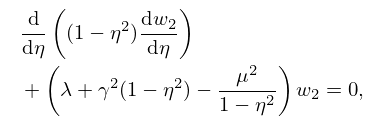
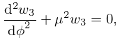
where , , satisfy the differential equations
| 30.13.9 | |||
| 30.13.10 | |||
| 30.13.11 | |||
with and separation constants and . Equations (30.13.9) and (30.13.10) agree with (30.2.1).
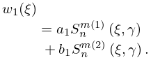
In most applications the solution has to be a single-valued function of , which requires (a nonnegative integer) and
| 30.13.12 | |||
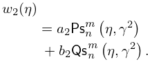
Moreover, has to be bounded along the -axis away from the focal line: this requires to be bounded when . Then for some , and the general solution of (30.13.10) is
| 30.13.13 | |||
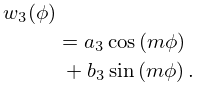
The solution of (30.13.9) with is
| 30.13.14 | |||
§30.13(v) The Interior Dirichlet Problem for Prolate Ellipsoids
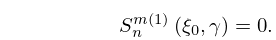
Equation (30.13.7) for , and subject to the boundary condition on the ellipsoid given by , poses an eigenvalue problem with as spectral parameter. The eigenvalues are given by , where is determined from the condition
| 30.13.15 | |||
The corresponding eigenfunctions are given by (30.13.8), (30.13.14), (30.13.13), (30.13.12), with . For the Dirichlet boundary-value problem of the region between two ellipsoids, the eigenvalues are determined from
| 30.13.16 | |||
with as in (30.13.14). The corresponding eigenfunctions are given as before with .
