日本金泽医科大学文凭毕业证哪里有卖【仿证 微kaa77788】】LeQ

SearchAdvancedHelp

The term"kaa77788" was not found.Possible alternative term: "27789".

(0.003 seconds)

1—10 of 316 matching pages

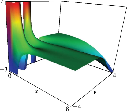
1: 28.21 Graphics

… ►

►

►

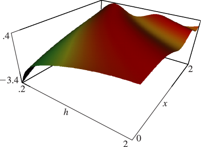
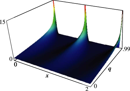
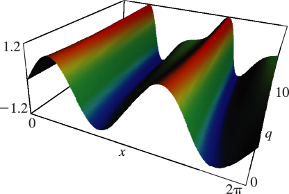
Figure 28.21.1: ${\mathrm{Mc}}_0^{(1)}(x,h)$ for $0\le h\le 3$, $0\le x\le 2$. Magnify 3D Help

►

►

►

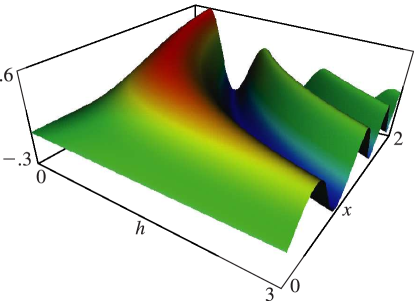
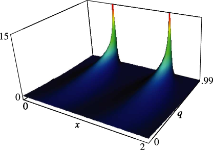
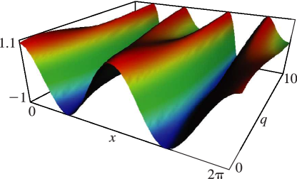
Figure 28.21.2: ${\mathrm{Mc}}_1^{(1)}(x,h)$ for $0\le h\le 3$, $0\le x\le 2$. Magnify 3D Help

►

►

►

Figure 28.21.3: ${\mathrm{Mc}}_0^{(2)}(x,h)$ for $0.1\le h\le 2$, $0\le x\le 2$. Magnify 3D Help

►

►

►

Figure 28.21.4: ${\mathrm{Mc}}_1^{(2)}(x,h)$ for $0.2\le h\le 2$, $0\le x\le 2$. Magnify 3D Help

►

►

►

Figure 28.21.5: ${\mathrm{Ms}}_1^{(1)}(x,h)$ for $0\le h\le 3$, $0\le x\le 2$. Magnify 3D Help

…

2: 20.3 Graphics

… ►

►

►

Figure 20.3.10: ${\theta }_1(\pi x,q)$, $0\le x\le 2$, $0\le q\le 0.99$. Magnify 3D Help

►

►

►

Figure 20.3.11: ${\theta }_2(\pi x,q)$, $0\le x\le 2$, $0\le q\le 0.99$. Magnify 3D Help

►

►

►

Figure 20.3.12: ${\theta }_3(\pi x,q)$, $0\le x\le 2$, $0\le q\le 0.99$. Magnify 3D Help

►

►

►

Figure 20.3.13: ${\theta }_4(\pi x,q)$, $0\le x\le 2$, $0\le q\le 0.99$. Magnify 3D Help

… ►

►

►

Figure 20.3.14: ${\theta }_1(\pi x+\mathrm{i}y,0.12)$, $-1\le x\le 1$, $-1\le y\le 2.3$. Magnify 3D Help

…

3: 7.3 Graphics

… ►

►►

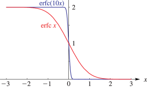
Figure 7.3.1: Complementary error functions $\mathrm{erfc}x$ and $\mathrm{erfc}\left(10x\right)$, $-3\le x\le 3$. Magnify

►

►►

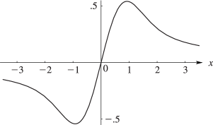
Figure 7.3.2: Dawson’s integral $F\left(x\right)$, $-3.5\le x\le 3.5$. Magnify

►

►►

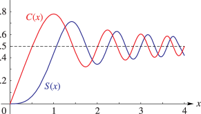
Figure 7.3.3: Fresnel integrals $C\left(x\right)$ and $S\left(x\right)$, $0\le x\le 4$. Magnify

… ►

►

►

Figure 7.3.5: $|\mathrm{erf}\left(x+\mathrm{i}y\right)|$, $-3\le x\le 3$, $-3\le y\le 3$. … Magnify 3D Help

►

►

►

Figure 7.3.6: $|\mathrm{erfc}\left(x+\mathrm{i}y\right)|$, $-3\le x\le 3$, $-3\le y\le 3$. … Magnify 3D Help

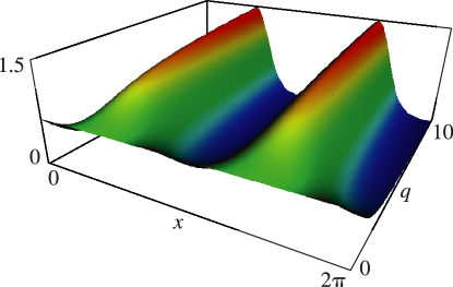
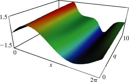
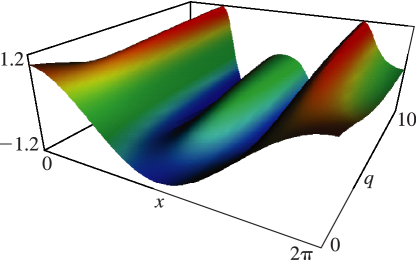
4: 14.22 Graphics

… ►

►

►

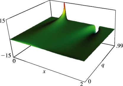
Figure 14.22.1: $P_{1/2}^0\left(x+\mathrm{i}y\right)$, $-5\le x\le 5$, $-5\le y\le 5$. … Magnify 3D Help

►

►

►

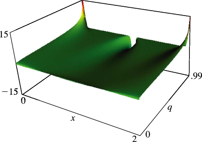
Figure 14.22.2: $P_{1/2}^{-1/2}\left(x+\mathrm{i}y\right)$, $-5\le x\le 5$, $-5\le y\le 5$. … Magnify 3D Help

►

►

►

Figure 14.22.3: $P_{1/2}^{-1}\left(x+\mathrm{i}y\right)$, $-5\le x\le 5$, $-5\le y\le 5$. … Magnify 3D Help

►

►

►

Figure 14.22.4: ${𝑸}_0^0\left(x+\mathrm{i}y\right)$, $-5\le x\le 5$, $-5\le y\le 5$. … Magnify 3D Help

5: 23.16 Graphics

… ►

►►

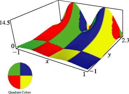
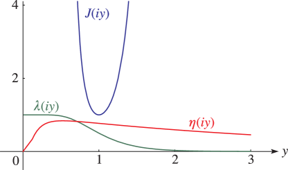
Figure 23.16.1: Modular functions $\lambda \left(\mathrm{i}y\right)$, $J\left(\mathrm{i}y\right)$, $\eta \left(\mathrm{i}y\right)$ for $0\le y\le 3$. … Magnify

►

►

►

Figure 23.16.2: Elliptic modular function $\lambda \left(x+\mathrm{i}y\right)$ for $-0.25\le x\le 0.25$, $0.005\le y\le 0.1$. Magnify 3D Help

►

►

►

Figure 23.16.3: Dedekind’s eta function $\eta \left(x+\mathrm{i}y\right)$ for $-0.0625\le x\le 0.0625$, $0.0001\le y\le 0.07$. Magnify 3D Help

6: 25.20 Approximations

… ►

Cody et al. (1971) gives rational approximations for $\zeta \left(s\right)$ in the form of quotients of polynomials or quotients of Chebyshev series. The ranges covered are $0.5\le s\le 5$, $5\le s\le 11$, $11\le s\le 25$, $25\le s\le 55$. Precision is varied, with a maximum of 20S.

►

Piessens and Branders (1972) gives the coefficients of the Chebyshev-series expansions of $s\zeta \left(s+1\right)$ and $\zeta \left(s+k\right)$, $k=2,3,4,5,8$, for $0\le s\le 1$ (23D).

►

Luke (1969b, p. 306) gives coefficients in Chebyshev-series expansions that cover $\zeta \left(s\right)$ for $0\le s\le 1$ (15D), $\zeta \left(s+1\right)$ for $0\le s\le 1$ (20D), and $\ln \xi \left(\frac{1}{2}+\mathrm{i}x\right)$ (§25.4) for $-1\le x\le 1$ (20D). For errata see Piessens and Branders (1972).

►

Morris (1979) gives rational approximations for ${\mathrm{Li}}_2\left(x\right)$ (§25.12(i)) for $0.5\le x\le 1$. Precision is varied with a maximum of 24S.

►

Antia (1993) gives minimax rational approximations for $\mathrm{\Gamma }\left(s+1\right)F_s(x)$, where $F_s(x)$ is the Fermi–Dirac integral (25.12.14), for the intervals and , with $s=-\frac{1}{2},\frac{1}{2},\frac{3}{2},\frac{5}{2}$. For each $s$ there are three sets of approximations, with relative maximum errors ${10}^{-4},{10}^{-8},{10}^{-12}$.

7: 10.3 Graphics

… ►

►

►

Figure 10.3.5: $J_{\nu }\left(x\right)$, $0\le x\le 10$, $0\le \nu \le 5$. Magnify 3D Help

… ►

►

►

Figure 10.3.7: $J_{\nu }^{\prime }\left(x\right)$, $0\le x\le 10$, $0\le \nu \le 5$. Magnify 3D Help

►

►

►

Figure 10.3.8: $Y_{\nu }^{\prime }\left(x\right)$, $0.2\le x\le 10$, $0\le \nu \le 5$. Magnify 3D Help

… ►

►

►

Figure 10.3.9: $J_0\left(x+\mathrm{i}y\right)$, $-10\le x\le 10$, $-4\le y\le 4$. Magnify 3D Help

… ►

►

►

Figure 10.3.11: $J_1\left(x+\mathrm{i}y\right)$, $-10\le x\le 10$, $-4\le y\le 4$. Magnify 3D Help

…

8: 11.3 Graphics

… ►

►

►

Figure 11.3.5: ${𝐇}_{\nu }\left(x\right)$ for $0\le x\le 8$ and $-4\le \nu \le 4$. Magnify 3D Help

►

►

►

Figure 11.3.6: ${𝐊}_{\nu }\left(x\right)$ for $0\le x\le 8$ and $-4\le \nu \le 4$. Magnify 3D Help

►

►

►

Figure 11.3.7: $\left|{𝐇}_0\left(x+\mathrm{i}y\right)\right|$ for $-8\le x\le 8$ and $-3\le y\le 3$. Magnify 3D Help

… ►

►

►

Figure 11.3.17: ${𝐋}_{\nu }\left(x\right)$ for $0\le x\le 5.6$ and $-4\le \nu \le 4$. Magnify 3D Help

►

►

►

Figure 11.3.18: ${𝐌}_{\nu }\left(x\right)$ for $0\le x\le 8$ and $-4\le \nu \le 4$. Magnify 3D Help

…

9: 28.3 Graphics

… ►

►

►

Figure 28.3.9: ${\mathrm{ce}}_0(x,q)$ for $0\le x\le 2\pi$, $0\le q\le 10$. Magnify 3D Help

►

►

►

Figure 28.3.10: ${\mathrm{se}}_1(x,q)$ for $0\le x\le 2\pi$, $0\le q\le 10$. Magnify 3D Help

►

►

►

Figure 28.3.11: ${\mathrm{ce}}_1(x,q)$ for $0\le x\le 2\pi$, $0\le q\le 10$. Magnify 3D Help

►

►

►

Figure 28.3.12: ${\mathrm{se}}_2(x,q)$ for $0\le x\le 2\pi$, $0\le q\le 10$. Magnify 3D Help

►

►

►

Figure 28.3.13: ${\mathrm{ce}}_2(x,q)$ for $0\le x\le 2\pi$, $0\le q\le 10$. Magnify 3D Help

10: 25.3 Graphics

… ►

►►

Figure 25.3.1: Riemann zeta function $\zeta \left(x\right)$ and its derivative ${\zeta }^{\prime }\left(x\right)$, $-20\le x\le 10$. Magnify

… ►

►

►

Figure 25.3.3: Modulus of the Riemann zeta function $|\zeta \left(x+\mathrm{i}y\right)|$, $-4\le x\le 4$, $-10\le y\le 40$. Magnify 3D Help

►

►►

Figure 25.3.4: $Z(t)$, $0\le t\le 50$. … Magnify

►

►►

Figure 25.3.5: $Z(t)$, $1000\le t\le 1050$. Magnify

►

►►

Figure 25.3.6: $Z(t)$, $10000\le t\le 10050$. Magnify