with imaginary periods

SearchAdvancedHelp

(0.002 seconds)

31—40 of 40 matching pages

31: 22.19 Physical Applications

… ►The period is $4K\left(\sin \left(\frac{1}{2}\alpha \right)\right)$. … ►Figure 22.19.1 shows the nature of the solutions $\theta (t)$ of (22.19.3) by graphing $\mathrm{am}(x,k)$ for both $0\le k\le 1$, as in Figure 22.16.1, and $k\ge 1$, where it is periodic. … ►As $a\to \sqrt{1/\beta }$ from below the period diverges since $a=\pm \sqrt{1/\beta }$ are points of unstable equilibrium. … ►Such oscillations, of period $2K\left(k\right)/\sqrt{\eta }$, with modulus $k=1/\sqrt{2-{\eta }^{-1}}$ are given by: …As $a\to \sqrt{2/\beta }$ from below the period diverges since $x=0$ is a point of unstable equlilibrium. …

32: 3.4 Differentiation

… ►

3.4.17 $$\frac{1}{k!}{f}^{(k)}(x_0)=\frac{1}{2\pi \mathrm{i}}{\int }_C\frac{f(\zeta )}{{(\zeta -x_0)}^{k+1}}d\zeta ,$$

ⓘ

Symbols:

$\pi$: the ratio of the circumference of a circle to its diameter, $dx$: differential of $x$ , $!$: factorial (as in $n!$), $\mathrm{i}$: imaginary unit, $\int$: integral and $C$: simple closed contour

Permalink:

http://dlmf.nist.gov/3.4.E17

Encodings:

pMML, png, TeX

See also:

Annotations for §3.4(ii), §3.4 and Ch.3

… ►

3.4.18 $$\frac{1}{k!}{f}^{(k)}(x_0)=\frac{1}{2\pi r^k}{\int }_0^{2\pi }f(x_0+r{\mathrm{e}}^{\mathrm{i}\theta }){\mathrm{e}}^{-\mathrm{i}k\theta }d\theta .$$

ⓘ

Symbols:

$\pi$: the ratio of the circumference of a circle to its diameter, $dx$: differential of $x$ , $\mathrm{e}$: base of natural logarithm, $!$: factorial (as in $n!$), $\mathrm{i}$: imaginary unit, $\int$: integral and $r$: radius

Referenced by:

§3.4(ii)

Permalink:

http://dlmf.nist.gov/3.4.E18

Encodings:

pMML, png, TeX

See also:

Annotations for §3.4(ii), §3.4 and Ch.3

… ►As explained in §§3.5(i) and 3.5(ix) the composite trapezoidal rule can be very efficient for computing integrals with analytic periodic integrands. …

33: 22.2 Definitions

… ►As a function of $z$, with fixed $k$, each of the 12 Jacobian elliptic functions is doubly periodic, having two periods whose ratio is not real. … … ►

22.2.12 $$\tau =\mathrm{i}{K}^{\prime }\left(k\right)/K\left(k\right),$$

ⓘ

Symbols:

$K^{\prime }\left(k\right)$: Legendre’s complementary complete elliptic integral of the first kind, $K\left(k\right)$: Legendre’s complete elliptic integral of the first kind, $\mathrm{i}$: imaginary unit, $k$: modulus and $\tau$: ratio

Referenced by:

§22.2

Permalink:

http://dlmf.nist.gov/22.2.E12

Encodings:

pMML, png, TeX

See also:

Annotations for §22.2, §22.2 and Ch.22

…

34: Bibliography I

… ►

The periodic Lamé functions. Proc. Roy. Soc. Edinburgh 60, pp. 47–63.

ⓘ

External Links:

MathReview (H. Bateman), ZentralBlatt

Referenced by:

§29.1, §29.15(ii), 1st item, §29.7(i).

Encodings:

BibTeX

►

Further investigations into the periodic Lamé functions. Proc. Roy. Soc. Edinburgh 60, pp. 83–99.

ⓘ

External Links:

MathReview (H. Bateman), ZentralBlatt

Referenced by:

§29.1, §29.17(ii), §29.3(iii), §29.6(i), §29.6(ii), §29.6(iii), §29.6(iv), Ch.29, Notations E, Notations E, Notations E, Notations E.

Encodings:

BibTeX

… ►

Bounds for the small real and purely imaginary zeros of Bessel and related functions. Methods Appl. Anal. 2 (1), pp. 1–21.

ⓘ

External Links:

ISSN 1073-2772, FullText, MathReview (Andrea Laforgia), ZentralBlatt

Referenced by:

§10.21(v).

Encodings:

BibTeX

…

35: 22.3 Graphics

… ►The period diverges logarithmically as $k\to 1-$; see §19.12. … ►

►►

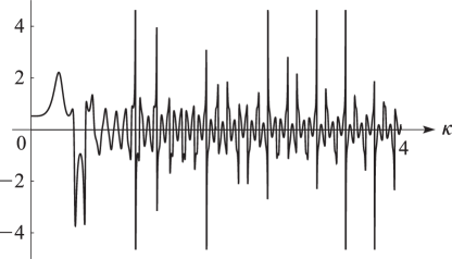
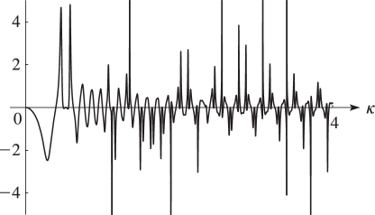
Figure 22.3.22: $\mathrm{\Re }\mathrm{sn}(x,k)$, $x=120$, as a function of $k^2=\mathrm{i}{\kappa }^2$, $0\le \kappa \le 4$. Magnify

►

►►

Figure 22.3.23: $\mathrm{\Im }\mathrm{sn}(x,k)$, $x=120$, as a function of $k^2=\mathrm{i}{\kappa }^2$, $0\le \kappa \le 4$. Magnify

… ►

►

►

Figure 22.3.24: $\mathrm{sn}(x+\mathrm{i}y,k)$ for $-4\le x\le 4$, $0\le y\le 8$, $k=1+\frac{1}{2}\mathrm{i}$. $K=1.5149\mathrm{\dots }+\mathrm{i}0.5235\mathrm{\dots }$, $K^{\prime }=1.4620\mathrm{\dots }-\mathrm{i}0.3552\mathrm{\dots }$. Magnify 3D Help

…

36: 28.32 Mathematical Applications

… ►This leads to integral equations and an integral relation between the solutions of Mathieu’s equation (setting $\zeta =\mathrm{i}\xi$, $z=\eta$ in (28.32.3)). … ►The first is the $2\pi$-periodicity of the solutions; the second can be their asymptotic form. …

37: 1.14 Integral Transforms

… ►(Some references replace $\mathrm{i}xt$ by $-\mathrm{i}xt$). … ►

Periodic Functions

… ►If $f(x)$ is continuous on $(0,\mathrm{\infty })$ and $ℳf\left(\sigma +\mathrm{i}t\right)$ is integrable on $(-\mathrm{\infty },\mathrm{\infty })$, then … ►Suppose $x^{-\sigma }f(x)$ and $x^{\sigma -1}g(x)$ are absolutely integrable on $(0,\mathrm{\infty })$ and either $ℳg\left(\sigma +\mathrm{i}t\right)$ or $ℳf\left(1-\sigma -\mathrm{i}t\right)$ is absolutely integrable on $(-\mathrm{\infty },\mathrm{\infty })$. … ►If $x^{\sigma -1}f(x)$ and $x^{\sigma -1}g(x)$ are absolutely integrable on $(0,\mathrm{\infty })$, then for $s=\sigma +\mathrm{i}t$, …

38: Bibliography G

… ►

Riemann surfaces, plane algebraic curves and their period matrices. J. Symbolic Comput. 26 (6), pp. 789–803.

ⓘ

External Links:

ISSN 0747-7171, Document, MathReview (Gabino González Díez), ZentralBlatt

Referenced by:

1st item.

Encodings:

BibTeX

… ►

Evaluation of the modified Bessel function of the third kind of imaginary orders. J. Comput. Phys. 175 (2), pp. 398–411.

ⓘ

External Links:

ISSN 0021-9991, Document, MathReview (J. P. Singhal), ZentralBlatt

Referenced by:

§10.74(viii).

Encodings:

BibTeX

►

Computation of the modified Bessel function of the third kind of imaginary orders: Uniform Airy-type asymptotic expansion. J. Comput. Appl. Math. 153 (1-2), pp. 225–234.

ⓘ

External Links:

ISSN 0377-0427, Document, MathReview, ZentralBlatt

Referenced by:

§10.45, §10.74(viii).

Encodings:

BibTeX

… ►

Algorithm 831: Modified Bessel functions of imaginary order and positive argument. ACM Trans. Math. Software 30 (2), pp. 159–164.

ⓘ

External Links:

ISSN 0098-3500, Document, GAMS (module 831; package TOMS), MathReview Entry, ZentralBlatt

Referenced by:

1st item.

Encodings:

BibTeX

►

Computing solutions of the modified Bessel differential equation for imaginary orders and positive arguments. ACM Trans. Math. Software 30 (2), pp. 145–158.

ⓘ

External Links:

ISSN 0098-3500, Document, MathReview, ZentralBlatt

Referenced by:

§10.74(viii).

Encodings:

BibTeX

…

39: 23.6 Relations to Other Functions

… ►

$q={\mathrm{e}}^{\mathrm{i}\pi \tau },$

… ►Also, ${𝕃}_1$, ${𝕃}_2$, ${𝕃}_3$ are the lattices with generators $(4K,2\mathrm{i}{K}^{\prime })$, $(2K-2\mathrm{i}{K}^{\prime },2K+2\mathrm{i}{K}^{\prime })$, $(2K,4\mathrm{i}{K}^{\prime })$, respectively. … ►

23.6.31 $$z-{\omega }_1=\frac{\mathrm{i}}{2}{\int }_t^{e_1}\frac{du}{\sqrt{(e_1-u)(u-e_2)(u-e_3)}},$$ $e_2\le t\le e_1$, $z\in [{\omega }_1,{\omega }_1+{\omega }_3]$,

ⓘ

Symbols:

$e_j$: Weierstrass lattice roots, $[a,b]$: closed interval, $dx$: differential of $x$ , $\in$: element of, $\mathrm{i}$: imaginary unit, $\int$: integral, $𝕃$: lattice, $z$: complex, ${\omega }_1$, ${\omega }_3$, ${\omega }_2=-{\omega }_1-{\omega }_3$: lattice generators and $t$

Permalink:

http://dlmf.nist.gov/23.6.E31

Encodings:

pMML, png, TeX

See also:

Annotations for §23.6(iv), §23.6(iv), §23.6 and Ch.23

… ►

23.6.33 $$z=\frac{\mathrm{i}}{2}{\int }_{-\mathrm{\infty }}^t\frac{du}{\sqrt{(e_1-u)(e_2-u)(e_3-u)}},$$ $t\le e_3$, $z\in (0,{\omega }_3]$.

ⓘ

Symbols:

$e_j$: Weierstrass lattice roots, $dx$: differential of $x$ , $\in$: element of, $\mathrm{i}$: imaginary unit, $\int$: integral, $(a,b]$: half-closed interval, $𝕃$: lattice, $z$: complex, ${\omega }_1$, ${\omega }_3$, ${\omega }_2=-{\omega }_1-{\omega }_3$: lattice generators and $t$

Permalink:

http://dlmf.nist.gov/23.6.E33

Encodings:

pMML, png, TeX

See also:

Annotations for §23.6(iv), §23.6(iv), §23.6 and Ch.23

… ►

23.6.35 $$2{\omega }_3=\mathrm{i}{\int }_{e_2}^{e_1}\frac{du}{\sqrt{(e_1-u)(u-e_2)(u-e_3)}}=\mathrm{i}{\int }_{-\mathrm{\infty }}^{e_3}\frac{du}{\sqrt{(e_1-u)(e_2-u)(e_3-u)}}.$$

ⓘ

Symbols:

$e_j$: Weierstrass lattice roots, $dx$: differential of $x$ , $\mathrm{i}$: imaginary unit, $\int$: integral, $𝕃$: lattice and ${\omega }_1$, ${\omega }_3$, ${\omega }_2=-{\omega }_1-{\omega }_3$: lattice generators

Referenced by:

§23.6(iv)

Permalink:

http://dlmf.nist.gov/23.6.E35

Encodings:

pMML, png, TeX

See also:

Annotations for §23.6(iv), §23.6(iv), §23.6 and Ch.23

…

40: Errata

… ►

A phrase was added, just below (1.9.1), which elaborates that ${\mathrm{i}}^2=-1$.

… ►

To be consistent with the notation used in (8.12.16), Equation (8.12.5) was changed to read

8.12.5 $$\frac{{\mathrm{e}}^{\pm \pi \mathrm{i}a}}{2\mathrm{i}\sin (\pi a)}Q(-a,z{\mathrm{e}}^{\pm \pi \mathrm{i}})=\pm \frac{1}{2}\mathrm{erfc}\left(\pm \mathrm{i}\eta \sqrt{a/2}\right)-\mathrm{i}T(a,\eta )$$

… ►

Originally all six integrands in these equations were incorrect because their numerators contained the function ${\tilde{B}}_2\left(x\right)$. The correct function is $\frac{{\tilde{B}}_2\left(x\right)-B_2}{2}$. The new equations are:

25.11.6 $$\zeta (s,a)=\frac{1}{a^s}\left(\frac{1}{2}+\frac{a}{s-1}\right)-\frac{s(s+1)}{2}{\int }_0^{\mathrm{\infty }}\frac{{\tilde{B}}_2\left(x\right)-B_2}{{(x+a)}^{s+2}}dx,$$ $s\ne 1$, $\mathrm{\Re }s>-1$, $a>0$

Reported 2016-05-08 by Clemens Heuberger.

25.11.19 $${\zeta }^{\prime }(s,a)=-\frac{\ln a}{a^s}\left(\frac{1}{2}+\frac{a}{s-1}\right)-\frac{a^{1-s}}{{(s-1)}^2}+\frac{s(s+1)}{2}{\int }_0^{\mathrm{\infty }}\frac{({\tilde{B}}_2\left(x\right)-B_2)\ln \left(x+a\right)}{{(x+a)}^{s+2}}dx-\frac{(2s+1)}{2}{\int }_0^{\mathrm{\infty }}\frac{{\tilde{B}}_2\left(x\right)-B_2}{{(x+a)}^{s+2}}dx,$$ $\mathrm{\Re }s>-1$, $s\ne 1$, $a>0$

Reported 2016-06-27 by Gergő Nemes.

25.11.20 $${(-1)}^k{\zeta }^{(k)}(s,a)=\frac{{(\ln a)}^k}{a^s}\left(\frac{1}{2}+\frac{a}{s-1}\right)+k!a^{1-s}\sum _{r=0}^{k-1}\frac{{(\ln a)}^r}{r!{(s-1)}^{k-r+1}}-\frac{s(s+1)}{2}{\int }_0^{\mathrm{\infty }}\frac{({\tilde{B}}_2\left(x\right)-B_2){(\ln \left(x+a\right))}^k}{{(x+a)}^{s+2}}dx+\frac{k(2s+1)}{2}{\int }_0^{\mathrm{\infty }}\frac{({\tilde{B}}_2\left(x\right)-B_2){(\ln \left(x+a\right))}^{k-1}}{{(x+a)}^{s+2}}dx-\frac{k(k-1)}{2}{\int }_0^{\mathrm{\infty }}\frac{({\tilde{B}}_2\left(x\right)-B_2){(\ln \left(x+a\right))}^{k-2}}{{(x+a)}^{s+2}}dx,$$ $\mathrm{\Re }s>-1$, $s\ne 1$, $a>0$

Reported 2016-06-27 by Gergő Nemes.

… ►

We avoid the troublesome symbols, often missing in installed fonts, previously used for exponential $\mathrm{e}$, imaginary $\mathrm{i}$ and differential $d$.

… ►

The captions for these figures have been corrected to read, in part, “as a function of $k^2=\mathrm{i}{\kappa }^2$” (instead of $k^2=\mathrm{i}\kappa$). Also, the resolution of the graph in Figure 22.3.22 was improved near $\kappa =3$.

Reported 2011-10-30 by Paul Abbott.

…