with%20a%20parameter

SearchAdvancedHelp

(0.007 seconds)

11—20 of 37 matching pages

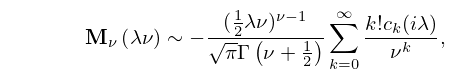
11: 28.8 Asymptotic Expansions for Large $q$

… ►

28.8.1 $$\begin{array}{c}{a}_m\left(h^2\right)\\ b_{m+1}\left(h^2\right)\end{array}\}\sim -2h^2+2sh-\frac{1}{8}(s^2+1)-\frac{1}{2^{7}h}(s^3+3s)-\frac{1}{2^{12}{h}^2}(5s^4+34s^2+9)-\frac{1}{2^{17}{h}^3}(33s^5+410s^3+405s)-\frac{1}{2^{20}{h}^4}(63s^6+1260s^4+2943s^2+486)-\frac{1}{2^{25}{h}^5}(527s^7+15617s^5+69001s^3+41607s)+\mathrm{\cdots }.$$

ⓘ

Symbols:

$a_n\left(q\right)$: eigenvalues of Mathieu equation, $b_n\left(q\right)$: eigenvalues of Mathieu equation, $\sim$: Poincaré asymptotic expansion, $m$: integer and $h$: parameter

A&S Ref:

20.2.30 (in different form)

Referenced by:

§28.8(i), Erratum (V1.1.10) for Sections 28.6(i), 28.6(ii), 28.8(i), 28.8(ii)

Permalink:

http://dlmf.nist.gov/28.8.E1

Encodings:

pMML, png, TeX

See also:

Annotations for §28.8(i), §28.8 and Ch.28

…

12: Bibliography M

… ►

Rational approximations, software and test methods for sine and cosine integrals. Numer. Algorithms 12 (3-4), pp. 259–272.

ⓘ

Notes:

Includes Fortran code, maximum accuracy 20S.

External Links:

ISSN 1017-1398, Document, MathReview, ZentralBlatt

Referenced by:

§6.13, 4th item, §6.21(ii).

Encodings:

BibTeX

… ►

On one-parameter families of Painlevé III. Stud. Appl. Math. 101 (3), pp. 321–341.

ⓘ

External Links:

ISSN 0022-2526, Document, MathReview (Andrei A. Kapaev), ZentralBlatt

Referenced by:

§32.10(iii).

Encodings:

BibTeX

… ►

Hierarchies and logarithmic oscillations in the temporal relaxation patterns of proteins and other complex systems. Proc. Nat. Acad. Sci. U .S. A. 96 (20), pp. 11085–11089.

ⓘ

External Links:

FullText

Referenced by:

§8.24(i).

Encodings:

BibTeX

… ►

The $q$-analogue of the Laguerre polynomials. J. Math. Anal. Appl. 81 (1), pp. 20–47.

ⓘ

External Links:

ISSN 0022-247X, Document, MathReview (R. A. Askey), ZentralBlatt

Referenced by:

§18.27(v).

Encodings:

BibTeX

… ►

Tables of the functions of the parabolic cylinder for negative integer parameters. Zastos. Mat. 13, pp. 261–273.

ⓘ

External Links:

MathReview, ZentralBlatt

Referenced by:

7th item.

Encodings:

BibTeX

…

13: Bibliography O

… ►

Uniform asymptotic expansions for hypergeometric functions with large parameters. I. Analysis and Applications (Singapore) 1 (1), pp. 111–120.

ⓘ

External Links:

ISSN 0219-5305, Document, MathReview, ZentralBlatt

Referenced by:

§15.12(iii).

Encodings:

BibTeX

►

Uniform asymptotic expansions for hypergeometric functions with large parameters. II. Analysis and Applications (Singapore) 1 (1), pp. 121–128.

ⓘ

External Links:

ISSN 0219-5305, Document, MathReview, ZentralBlatt

Referenced by:

§15.12(iii).

Encodings:

BibTeX

… ►

Uniform asymptotic expansions for hypergeometric functions with large parameters. III. Analysis and Applications (Singapore) 8 (2), pp. 199–210.

ⓘ

External Links:

ISSN 0219-5305, Document, MathReview (Javier Segura), ZentralBlatt

Referenced by:

§15.12(iii).

Encodings:

BibTeX

… ►

Legendre functions with both parameters large. Philos. Trans. Roy. Soc. London Ser. A 278, pp. 175–185.

ⓘ

External Links:

FullText, MathReview (P. F. Hsieh), ZentralBlatt

Referenced by:

§14.15(v), §14.15(v).

Encodings:

BibTeX

… ►

Whittaker functions with both parameters large: Uniform approximations in terms of parabolic cylinder functions. Proc. Roy. Soc. Edinburgh Sect. A 86 (3-4), pp. 213–234.

ⓘ

External Links:

ISSN 0308-2105, MathReview (P. F. Hsieh), ZentralBlatt

Referenced by:

§13.20(iii), §13.20(iv).

Encodings:

BibTeX

…

14: 11.6 Asymptotic Expansions

… ►For fixed $\lambda (>1)$ ►

11.6.6 $${𝐊}_{\nu }\left(\lambda \nu \right)\sim \frac{{(\frac{1}{2}\lambda \nu )}^{\nu -1}}{\sqrt{\pi }\mathrm{\Gamma }\left(\nu +\frac{1}{2}\right)}\sum _{k=0}^{\mathrm{\infty }}\frac{k!c_k(\lambda )}{{\nu }^k},$$ $|\mathrm{ph}\nu |\le \frac{1}{2}\pi -\delta$,

ⓘ

Symbols:

$\mathrm{\Gamma }\left(z\right)$: gamma function, ${𝐊}_{\nu }\left(z\right)$: Struve function, $\sim$: Poincaré asymptotic expansion, $\pi$: the ratio of the circumference of a circle to its diameter, $!$: factorial (as in $n!$), $\mathrm{ph}$: phase, $\nu$: real or complex order, $k$: nonnegative integer, $\delta$: arbitrary small positive constant, $\lambda$: parameter and $c_k(\lambda )$: expansion function

A&S Ref:

12.1.34

Referenced by:

§11.6(iii)

Permalink:

http://dlmf.nist.gov/11.6.E6

Encodings:

pMML, png, TeX

See also:

Annotations for §11.6(iii), §11.6 and Ch.11

… ►

11.6.7 $${𝐌}_{\nu }\left(\lambda \nu \right)\sim -\frac{{(\frac{1}{2}\lambda \nu )}^{\nu -1}}{\sqrt{\pi }\mathrm{\Gamma }\left(\nu +\frac{1}{2}\right)}\sum _{k=0}^{\mathrm{\infty }}\frac{k!c_k(\mathrm{i}\lambda )}{{\nu }^k},$$ $|\mathrm{ph}\nu |\le \frac{1}{2}\pi -\delta$.

ⓘ

Symbols:

$\mathrm{\Gamma }\left(z\right)$: gamma function, ${𝐌}_{\nu }\left(z\right)$: modified Struve function, $\sim$: Poincaré asymptotic expansion, $\pi$: the ratio of the circumference of a circle to its diameter, $!$: factorial (as in $n!$), $\mathrm{i}$: imaginary unit, $\mathrm{ph}$: phase, $\nu$: real or complex order, $k$: nonnegative integer, $\delta$: arbitrary small positive constant, $\lambda$: parameter and $c_k(\lambda )$: expansion function

Referenced by:

§11.6(iii)

Permalink:

http://dlmf.nist.gov/11.6.E7

Encodings:

pMML, png, TeX

See also:

Annotations for §11.6(iii), §11.6 and Ch.11

… ►

$c_3(\lambda )=20{\lambda }^{-6}-4{\lambda }^{-4},$

… ►

11.6.9 $${𝐋}_{\nu }\left(\lambda \nu \right)\sim I_{\nu }\left(\lambda \nu \right),$$ $|\mathrm{ph}\nu |\le \frac{1}{2}\pi -\delta$,

ⓘ

Symbols:

$\sim$: asymptotic equality, $\pi$: the ratio of the circumference of a circle to its diameter, $I_{\nu }\left(z\right)$: modified Bessel function of the first kind, ${𝐋}_{\nu }\left(z\right)$: modified Struve function, $\mathrm{ph}$: phase, $\nu$: real or complex order, $\delta$: arbitrary small positive constant and $\lambda$: parameter

Referenced by:

§11.6(iii)

Permalink:

http://dlmf.nist.gov/11.6.E9

Encodings:

pMML, png, TeX

See also:

Annotations for §11.6(iii), §11.6 and Ch.11

…

15: 36.5 Stokes Sets

… ►where $j$ denotes a real critical point (36.4.1) or (36.4.2), and $\mu$ denotes a critical point with complex $t$ or $s,t$, connected with $j$ by a steepest-descent path (that is, a path where $\mathrm{\Re }\mathrm{\Phi }=\mathrm{constant}$) in complex $t$ or $(s,t)$ space. … ►The Stokes set is itself a cusped curve, connected to the cusp of the bifurcation set: … ►They generate a pair of cusp-edged sheets connected to the cusped sheets of the swallowtail bifurcation set (§36.4). … ►The first sheet corresponds to and is generated as a solution of Equations (36.5.6)–(36.5.9). … ►This consists of a cusp-edged sheet connected to the cusp-edged sheet of the bifurcation set and intersecting the smooth sheet of the bifurcation set. …

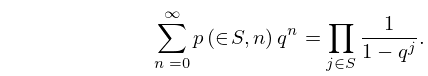
16: 26.10 Integer Partitions: Other Restrictions

… ►The set $\{n\ge 1|n\equiv \pm j(modk)\}$ is denoted by $A_{j,k}$. … ►

26.10.5 $$\sum _{n=0}^{\mathrm{\infty }}p(\in S,n)q^n=\prod _{j\in S}\frac{1}{1-q^j}.$$

ⓘ

Symbols:

$\in$: element of, $p(\mathrm{condition},n)$: restricted number of partitions of $n$ , $j$: nonnegative integer, $n$: nonnegative integer, $S$: set and $q$: parameter

Permalink:

http://dlmf.nist.gov/26.10.E5

Encodings:

pMML, png, TeX

See also:

Annotations for §26.10(ii), §26.10 and Ch.26

… ►It is known that for $k>3$, $p(𝒟k,n)\ge p(\in A_{1,k+3},n)$, with strict inequality for $n$ sufficiently large, provided that $k=2^m-1,m=3,4,5$, or $k\ge 32$; see Yee (2004). … ►where $I_1\left(x\right)$ is the modified Bessel function (§10.25(ii)), and …The quantity $A_k(n)$ is real-valued. …

17: 12.10 Uniform Asymptotic Expansions for Large Parameter

§12.10 Uniform Asymptotic Expansions for Large Parameter

… ►In this section we give asymptotic expansions of PCFs for large values of the parameter $a$ that are uniform with respect to the variable $z$, when both $a$ and $z$ $(=x)$ are real. … ►

§12.10(ii) Negative $a$,

… ►

§12.10(vii) Negative $a$, . Expansions in Terms of Airy Functions

… ►

18: 8.17 Incomplete Beta Functions

… ►Throughout §§8.17 and 8.18 we assume that $a>0$, $b>0$, and $0\le x\le 1$. … ►Addendum: For a companion equation see (8.17.24). … ►For a historical profile of ${\mathrm{B}}_x(a,b)$ see Dutka (1981). … ►With $a>0$, $b>0$, and , … ►The expansion (8.17.22) converges rapidly for . …

19: 3.8 Nonlinear Equations

… ►Suppose $f(z)$ also depends on a parameter $\alpha$, denoted by $f(z,\alpha )$. Then the sensitivity of a simple zero $z$ to changes in $\alpha$ is given by … ►Consider $x=20$ and $j=19$. We have $p^{\prime }(20)=19!$ and $a_{19}=1+2+\mathrm{\cdots }+20=210$. … ►It is called a Julia set. …

20: 18.40 Methods of Computation

… ►

A numerical approach to the recursion coefficients and quadrature abscissas and weights

… ►Results of low ($2$ to $3$ decimal digits) precision for $w(x)$ are easily obtained for $N\sim 10$ to $20$. … ►The quadrature points and weights can be put to a more direct and efficient use. … ►Equation (18.40.7) provides step-histogram approximations to ${\int }_a^{x}d\mu (x)$, as shown in Figure 18.40.1 for $N=12$ and $120$, shown here for the repulsive Coulomb–Pollaczek OP’s of Figure 18.39.2, with the parameters as listed therein. … ►In Figure 18.40.2 the approximations were carried out with a precision of 50 decimal digits.