vector
(0.001 seconds)
1—10 of 36 matching pages
1: 1.6 Vectors and Vector-Valued Functions
§1.6 Vectors and Vector-Valued Functions
►§1.6(i) Vectors
… ►Unit Vectors
… ►Cross Product (or Vector Product)
… ►§1.6(ii) Vectors: Alternative Notations
…2: 1.2 Elementary Algebra
…
►
§1.2(v) Matrices, Vectors, Scalar Products, and Norms
… ►Row and Column Vectors
… ►and the corresponding transposed row vector of length is … ►Two vectors and are orthogonal if … ►Vector Norms
…3: 1.1 Special Notation
…
►
►
…
| real variables. | |
| … | |
| inner, or scalar, product for real or complex vectors or functions. | |
| … | |
| , | column vectors. |
| the space of all -dimensional vectors. | |
| … | |
4: 1.18 Linear Second Order Differential Operators and Eigenfunction Expansions
…
►A complex linear vector space is called an inner product space if an inner product
is defined for all with the properties: (i) is complex linear in ; (ii) ; (iii) ; (iv) if then .
… becomes a normed linear vector space.
If then is normalized.
Two elements and in are orthogonal if .
…
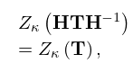
►The adjoint of does satisfy where .
…
5: 21.1 Special Notation
…
►
►
►Lowercase boldface letters or numbers are -dimensional real or complex vectors, either row or column depending on the context.
…
| positive integers. | |
| … | |
| -dimensional vectors, with all elements in , unless stated otherwise. | |
| th element of vector . | |
| … | |
| scalar product of the vectors and . | |
| … | |
| set of -dimensional vectors with elements in . | |
| … | |
6: 21.6 Products
…
►that is, is the number of elements in the set containing all -dimensional vectors obtained by multiplying on the right by a vector with integer elements.
Two such vectors are considered equivalent if their difference is a vector with integer elements.
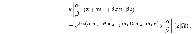
…where and are arbitrary -dimensional vectors.
…
►Then
…Thus is a -dimensional vector whose entries are either or .
…
7: 1.3 Determinants, Linear Operators, and Spectral Expansions
…
►
Linear Operators in Finite Dimensional Vector Spaces
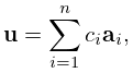
►Square matices can be seen as linear operators because for all and , the space of all -dimensional vectors. … ►The adjoint of a matrix is the matrix such that for all . … ►Assuming is an orthonormal basis in , any vector may be expanded as ►
1.3.20
.
…
8: 3.2 Linear Algebra
…
►
