symmetric elliptic%0Aintegrals
(0.002 seconds)
41—50 of 738 matching pages
41: 35.1 Special Notation
…
►
►
…
►Related notations for the Bessel functions are (Faraut and Korányi (1994, pp. 320–329)), (Terras (1988, pp. 49–64)), and (Faraut and Korányi (1994, pp. 357–358)).
| complex variables. | |
| … | |
| space of all real symmetric matrices. | |
| real symmetric matrices. | |
| … | |
| space of positive-definite real symmetric matrices. | |
| … | |
| complex symmetric matrix. | |
| … | |
42: 19.31 Probability Distributions
§19.31 Probability Distributions
…43: 22.8 Addition Theorems
§22.8 Addition Theorems
… ►§22.8(iii) Special Relations Between Arguments
… ►
22.8.23
…
►If sums/differences of the ’s are rational multiples of , then further relations follow.
…
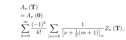
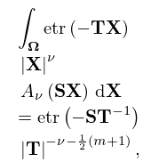
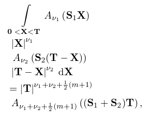
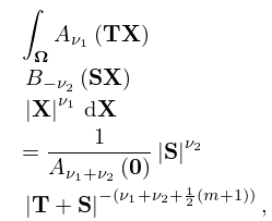
44: 35.5 Bessel Functions of Matrix Argument
45: 22.4 Periods, Poles, and Zeros
…
►
§22.4(i) Distribution
… ► … ►Figure 22.4.1 illustrates the locations in the -plane of the poles and zeros of the three principal Jacobian functions in the rectangle with vertices , , , . … ► … ►Figure 22.4.2 depicts the fundamental unit cell in the -plane, with vertices , , , . …46: 22.21 Tables
§22.21 Tables
►Spenceley and Spenceley (1947) tabulates , , , , for and to 12D, or 12 decimals of a radian in the case of . ►Curtis (1964b) tabulates , , for , , and (not ) to 20D. ►Lawden (1989, pp. 280–284 and 293–297) tabulates , , , , to 5D for , , where ranges from 1. … ►Zhang and Jin (1996, p. 678) tabulates , , for and to 7D. …47: 22.17 Moduli Outside the Interval [0,1]
§22.17 Moduli Outside the Interval [0,1]
►§22.17(i) Real or Purely Imaginary Moduli
►Jacobian elliptic functions with real moduli in the intervals and , or with purely imaginary moduli are related to functions with moduli in the interval by the following formulas. … ►§22.17(ii) Complex Moduli
… ►For proofs of these results and further information see Walker (2003).48: 23.6 Relations to Other Functions
…
►
§23.6(ii) Jacobian Elliptic Functions
… ►§23.6(iii) General Elliptic Functions
… ►§23.6(iv) Elliptic Integrals
… ►For relations to symmetric elliptic integrals see §19.25(vi). … ►49: 22.1 Special Notation
…
►
►
…
►The functions treated in this chapter are the three principal Jacobian elliptic functions , , ; the nine subsidiary Jacobian elliptic functions , , , , , , , , ; the amplitude function ; Jacobi’s epsilon and zeta functions and .
►The notation , , is due to Gudermann (1838), following Jacobi (1827); that for the subsidiary functions is due to Glaisher (1882).
Other notations for are and with ; see Abramowitz and Stegun (1964) and Walker (1996).
…
| real variables. | |
| … | |
| , | , (complete elliptic integrals of the first kind (§19.2(ii))). |
| … | |
