sine transform

SearchAdvancedHelp

(0.003 seconds)

11—20 of 56 matching pages

11: 20.10 Integrals

… ►

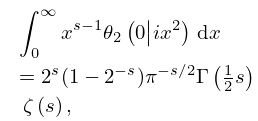
§20.10(i) Mellin Transforms with respect to the Lattice Parameter

►

20.10.1 $${\int }_0^{\mathrm{\infty }}{x}^{s-1}{\theta }_2\left(0\right|\mathrm{i}{x}^2)dx=2^s(1-2^{-s}){\pi }^{-s/2}\mathrm{\Gamma }\left(\frac{1}{2}s\right)\zeta \left(s\right),$$ $\mathrm{\Re }s>1$,

ⓘ

Symbols:

$\mathrm{\Gamma }\left(z\right)$: gamma function, ${\theta }_j\left(z\right|\tau )$: theta function, $\zeta \left(s\right)$: Riemann zeta function, $\pi$: the ratio of the circumference of a circle to its diameter, $dx$: differential of $x$ , $\mathrm{i}$: imaginary unit, $\int$: integral and $\mathrm{\Re }$: real part

Keywords:

Mellin transform

Referenced by:

§20.10(i), Erratum (V1.1.5) for §20.10(i)

Permalink:

http://dlmf.nist.gov/20.10.E1

Encodings:

pMML, png, TeX

Modification (effective with 1.1.5):

Originally the constraint was $\mathrm{\Re }s>2$. This can be relaxed to $\mathrm{\Re }s>1$ because ${\theta }_2\left(0\right|\mathrm{i}{x}^2)=x^{-1}{\theta }_4\left(0\right|\mathrm{i}{x}^{-2})\sim x^{-1}$ as $x\to 0+$, which follows from (20.7.31) and (20.4.5).

See also:

Annotations for §20.10(i), §20.10 and Ch.20

►

20.10.2 $${\int }_0^{\mathrm{\infty }}{x}^{s-1}({\theta }_3\left(0\right|\mathrm{i}{x}^2)-1)dx={\pi }^{-s/2}\mathrm{\Gamma }\left(\frac{1}{2}s\right)\zeta \left(s\right),$$ $\mathrm{\Re }s>1$,

ⓘ

Symbols:

$\mathrm{\Gamma }\left(z\right)$: gamma function, ${\theta }_j\left(z\right|\tau )$: theta function, $\zeta \left(s\right)$: Riemann zeta function, $\pi$: the ratio of the circumference of a circle to its diameter, $dx$: differential of $x$ , $\mathrm{i}$: imaginary unit, $\int$: integral and $\mathrm{\Re }$: real part

Keywords:

Mellin transform

Referenced by:

§20.10(i), Erratum (V1.1.5) for §20.10(i)

Permalink:

http://dlmf.nist.gov/20.10.E2

Encodings:

pMML, png, TeX

Modification (effective with 1.1.5):

Originally the constraint was $\mathrm{\Re }s>2$. This can be relaxed to $\mathrm{\Re }s>1$ because ${\theta }_3\left(0\right|\mathrm{i}{x}^2)=x^{-1}{\theta }_3\left(0\right|\mathrm{i}{x}^{-2})\sim x^{-1}$ as $x\to 0+$, which follows from (20.7.32) and (20.4.4).

See also:

Annotations for §20.10(i), §20.10 and Ch.20

… ►

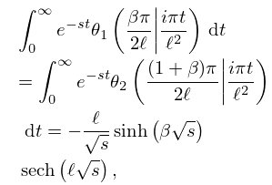
§20.10(ii) Laplace Transforms with respect to the Lattice Parameter

… ►

20.10.4 $${\int }_0^{\mathrm{\infty }}{\mathrm{e}}^{-st}{\theta }_1\left(\frac{\beta \pi }{2\mathrm{\ell }}\right|\frac{\mathrm{i}\pi t}{{\mathrm{\ell }}^2})dt={\int }_0^{\mathrm{\infty }}{\mathrm{e}}^{-st}{\theta }_2\left(\frac{(1+\beta )\pi }{2\mathrm{\ell }}\right|\frac{\mathrm{i}\pi t}{{\mathrm{\ell }}^2})dt=-\frac{\mathrm{\ell }}{\sqrt{s}}\sinh \left(\beta \sqrt{s}\right)\mathrm{sech}\left(\mathrm{\ell }\sqrt{s}\right),$$

ⓘ

Symbols:

${\theta }_j\left(z\right|\tau )$: theta function, $\pi$: the ratio of the circumference of a circle to its diameter, $dx$: differential of $x$ , $\mathrm{e}$: base of natural logarithm, $\mathrm{sech}z$: hyperbolic secant function, $\sinh z$: hyperbolic sine function, $\mathrm{i}$: imaginary unit, $\int$: integral, $s$: parameter, $\beta$: parameter and $\mathrm{\ell }$: parameter

Permalink:

http://dlmf.nist.gov/20.10.E4

Encodings:

pMML, png, TeX

See also:

Annotations for §20.10(ii), §20.10 and Ch.20

…

12: 19.8 Quadratic Transformations

… ►We consider only the descending Gauss transformation because its (ascending) inverse moves $F(\varphi ,k)$ closer to the singularity at $k=\sin \varphi =1$. …

13: 2.5 Mellin Transform Methods

… ►

2.5.9 $$ℳf\left(1-z\right)=\frac{\pi }{\sin \left(\pi z\right)},$$ ,

ⓘ

Symbols:

$ℳ\left(f\right)\left(s\right)$: Mellin transform, $\pi$: the ratio of the circumference of a circle to its diameter, $\mathrm{\Re }$: real part, $\sin z$: sine function and $f(t)=1/(1+t)$: function

Keywords:

Mellin transform

Permalink:

http://dlmf.nist.gov/2.5.E9

Encodings:

pMML, png, TeX

Notational Change (effective with 1.0.15):

The notation for the Mellin transform was changed to $ℳf\left(z\right)$ from $ℳ(f;z)$.

See also:

Annotations for §2.5(i), §2.5(i), §2.5 and Ch.2

►

2.5.10 $$ℳh\left(z\right)=\frac{2^{z-1}\mathrm{\Gamma }\left(\nu +\frac{1}{2}z\right)}{{\mathrm{\Gamma }}^2\left(1-\frac{1}{2}z\right)\mathrm{\Gamma }\left(1+\nu -\frac{1}{2}z\right)\mathrm{\Gamma }\left(z\right)}\frac{\pi }{\sin \left(\pi z\right)},$$ .

ⓘ

Symbols:

$\mathrm{\Gamma }\left(z\right)$: gamma function, $ℳ\left(f\right)\left(s\right)$: Mellin transform, $\pi$: the ratio of the circumference of a circle to its diameter, $\mathrm{\Re }$: real part, $\sin z$: sine function, $h(t)=J_{\nu }^2\left(t\right)$: function and $f(t)=1/(1+t)$: function

Keywords:

Mellin transform

Permalink:

http://dlmf.nist.gov/2.5.E10

Encodings:

pMML, png, TeX

Notational Change (effective with 1.0.15):

The notation for the Mellin transform was changed to $ℳf\left(z\right)$ from $ℳ(f;z)$.

See also:

Annotations for §2.5(i), §2.5(i), §2.5 and Ch.2

…

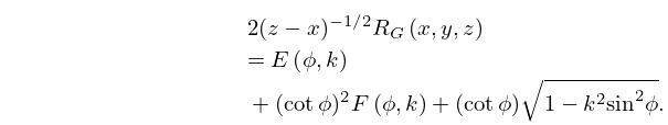
14: 19.25 Relations to Other Functions

… ►The transformations in §19.7(ii) result from the symmetry and homogeneity of functions on the right-hand sides of (19.25.5), (19.25.7), and (19.25.14). …then the five nontrivial permutations of $x,y,z$ that leave $R_F$ invariant change $k^2$ ($=(z-y)/(z-x)$) into $1/k^2$, $k_{}^{\prime }{}_{}{}^2$, $1/k_{}^{\prime }{}_{}{}^2$, $-k^2/k_{}^{\prime }{}_{}{}^2$, $-k_{}^{\prime }{}_{}{}^2/k^2$, and $\sin \varphi$ ($=\sqrt{(z-x)/z}$) into $k\sin \varphi$, $-\mathrm{i}\tan \varphi$, $-\mathrm{i}{k}^{\prime }\tan \varphi$, $(k^{\prime }\sin \varphi )/\sqrt{1-k^2{\sin }^2\varphi }$, $-\mathrm{i}k\sin \varphi /\sqrt{1-k^2{\sin }^2\varphi }$. Thus the five permutations induce five transformations of Legendre’s integrals (and also of the Jacobian elliptic functions). … ►

$\varphi =\arccos \sqrt{x/z}=\arcsin \sqrt{(z-x)/z},$

… ►

19.25.27 $$2{(z-x)}^{-1/2}{R}_G(x,y,z)=E(\varphi ,k)+{(\cot \varphi )}^{2}F(\varphi ,k)+(\cot \varphi )\sqrt{1-k^2{\sin }^2\varphi }.$$

ⓘ

Symbols:

$R_G(x,y,z)$: symmetric elliptic integral of second kind, $\cot z$: cotangent function, $F(\varphi ,k)$: Legendre’s incomplete elliptic integral of the first kind, $E(\varphi ,k)$: Legendre’s incomplete elliptic integral of the second kind, $\sin z$: sine function, $\varphi$: real or complex argument and $k$: real or complex modulus

Referenced by:

§19.25(iii)

Permalink:

http://dlmf.nist.gov/19.25.E27

Encodings:

pMML, png, TeX

See also:

Annotations for §19.25(iii), §19.25 and Ch.19

…

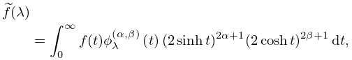
15: 15.9 Relations to Other Functions

… ►The Jacobi transform is defined as ►

15.9.12 $$\tilde{f}(\lambda )={\int }_0^{\mathrm{\infty }}f(t){\varphi }_{\lambda }^{(\alpha ,\beta )}\left(t\right){(2\sinh t)}^{2\alpha +1}{(2\cosh t)}^{2\beta +1}dt,$$

ⓘ

Symbols:

${\varphi }_{\lambda }^{(\alpha ,\beta )}\left(t\right)$: Jacobi function, $dx$: differential of $x$ , $\cosh z$: hyperbolic cosine function, $\sinh z$: hyperbolic sine function, $\int$: integral and $f(t)$: function

Permalink:

http://dlmf.nist.gov/15.9.E12

Encodings:

pMML, png, TeX

See also:

Annotations for §15.9(ii), §15.9 and Ch.15

►with inverse … … ►Any hypergeometric function for which a quadratic transformation exists can be expressed in terms of associated Legendre functions or Ferrers functions. …

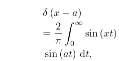
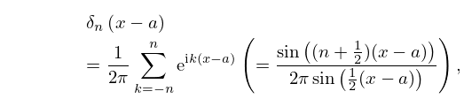
16: 1.17 Integral and Series Representations of the Dirac Delta

… ►

Sine and Cosine Functions

… ►

1.17.12_2 $$\delta \left(x-a\right)=\frac{2}{\pi }{\int }_0^{\mathrm{\infty }}\sin \left(xt\right)\sin \left(at\right)dt,$$ $x>0,a>0$.

ⓘ

Symbols:

$\delta \left(x-a\right)$: Dirac delta (or Dirac delta function), $\pi$: the ratio of the circumference of a circle to its diameter, $dx$: differential of $x$ , $\int$: integral and $\sin z$: sine function

Referenced by:

§1.17(ii), §1.17(ii), §1.17(ii), §1.18(vi), Erratum (V1.2.0) Section 1.17

Permalink:

http://dlmf.nist.gov/1.17.E12_2

Encodings:

pMML, png, TeX

See also:

Annotations for §1.17(ii), §1.17(ii), §1.17 and Ch.1

►Integral representation (1.17.12_1), (1.17.12_2) is the equivalent of the transform pairs, (1.14.9) (1.14.11), (1.14.10) (1.14.12), respectively. … ►

1.17.20 $${\delta }_n\left(x-a\right)=\frac{1}{2\pi }\sum _{k=-n}^n{\mathrm{e}}^{\mathrm{i}k(x-a)}\left(=\frac{\sin \left((n+\frac{1}{2})(x-a)\right)}{2\pi \sin \left(\frac{1}{2}(x-a)\right)}\right),$$

ⓘ

Symbols:

${\delta }_n\left(x\right)$: Dirac delta sequence, $\pi$: the ratio of the circumference of a circle to its diameter, $\mathrm{e}$: base of natural logarithm, $\mathrm{i}$: imaginary unit, $\sin z$: sine function, $k$: integer and $n$: nonnegative integer

Permalink:

http://dlmf.nist.gov/1.17.E20

Encodings:

pMML, png, TeX

See also:

Annotations for §1.17(iii), §1.17 and Ch.1

…

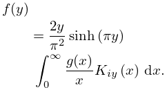
17: 10.43 Integrals

… ►

10.43.30 $$f(y)=\frac{2y}{{\pi }^2}\sinh \left(\pi y\right){\int }_0^{\mathrm{\infty }}\frac{g(x)}{x}{K}_{\mathrm{i}y}\left(x\right)dx.$$

ⓘ

Defines:

$f(x)$: Kontorovich–Lebedev transform of $g(x)$ (locally)

Symbols:

$\pi$: the ratio of the circumference of a circle to its diameter, $dx$: differential of $x$ , $\sinh z$: hyperbolic sine function, $\mathrm{i}$: imaginary unit, $\int$: integral, $K_{\nu }\left(z\right)$: modified Bessel function of the second kind, $x$: real variable, $y$: real variable and $g(x)$: function

Referenced by:

§10.43(v)

Permalink:

http://dlmf.nist.gov/10.43.E30

Encodings:

pMML, png, TeX

See also:

Annotations for §10.43(v), §10.43 and Ch.10

…

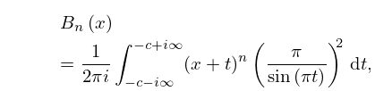
18: 24.7 Integral Representations

… ►

24.7.11 $$B_n\left(x\right)=\frac{1}{2\pi \mathrm{i}}{\int }_{-c-\mathrm{i}\mathrm{\infty }}^{-c+\mathrm{i}\mathrm{\infty }}{(x+t)}^n{\left(\frac{\pi }{\sin \left(\pi t\right)}\right)}^{2}dt,$$ .

ⓘ

Symbols:

$B_n\left(x\right)$: Bernoulli polynomials, $\pi$: the ratio of the circumference of a circle to its diameter, $dx$: differential of $x$ , $\mathrm{i}$: imaginary unit, $\int$: integral, $\sin z$: sine function, $n$: integer, $t$: real or complex and $x$: real or complex

Keywords:

Mellin transform

Referenced by:

§24.7(ii)

Permalink:

http://dlmf.nist.gov/24.7.E11

Encodings:

pMML, png, TeX

See also:

Annotations for §24.7(ii), §24.7(ii), §24.7 and Ch.24

…

19: 13.8 Asymptotic Approximations for Large Parameters

… ►When the foregoing results are combined with Kummer’s transformation (13.2.39), an approximation is obtained for the case when $|b|$ is large, and $|b-a|$ and $|z|$ are bounded. … ►where $w=\mathrm{arccosh}\left(1+{(2a)}^{-1}x\right)$, and $\beta =(w+\sinh w)/2$. …For the case $b>1$ the transformation (13.2.40) can be used. … ►

13.8.10 $$U(a,b,x)=\mathrm{\Gamma }\left(\frac{1}{2}b-a+\frac{1}{2}\right){\mathrm{e}}^{\frac{1}{2}x}{x}^{\frac{1}{2}-\frac{1}{2}b}\left(\cos \left(a\pi \right)J_{b-1}\left(\sqrt{2x(b-2a)}\right)-\sin \left(a\pi \right)Y_{b-1}\left(\sqrt{2x(b-2a)}\right)+\mathrm{env}{Y}_{b-1}\left(\sqrt{2x(b-2a)}\right)O\left({\left|a\right|}^{-\frac{1}{2}}\right)\right),$$

ⓘ

Symbols:

$J_{\nu }\left(z\right)$: Bessel function of the first kind, $Y_{\nu }\left(z\right)$: Bessel function of the second kind, $O\left(x\right)$: order not exceeding, $\mathrm{\Gamma }\left(z\right)$: gamma function, $U(a,b,z)$: Kummer confluent hypergeometric function, $\pi$: the ratio of the circumference of a circle to its diameter, $\cos z$: cosine function, $\mathrm{env}{Y}_{\nu }\left(x\right)$: envelope of Bessel function $Y_{\nu }\left(x\right)$ , $\mathrm{e}$: base of natural logarithm, $\sin z$: sine function and $x$: real variable

A&S Ref:

13.5.15 (in different form)

Referenced by:

§13.9(ii)

Permalink:

http://dlmf.nist.gov/13.8.E10

Encodings:

pMML, png, TeX

See also:

Annotations for §13.8(iii), §13.8 and Ch.13

… ►where $C_{\nu }(a,\zeta )=\cos \left(\pi a\right)J_{\nu }\left(\zeta \right)+\sin \left(\pi a\right)Y_{\nu }\left(\zeta \right)$ and …

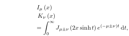
20: 10.32 Integral Representations

… ►

10.32.16 $$I_{\mu }\left(x\right)K_{\nu }\left(x\right)={\int }_0^{\mathrm{\infty }}{J}_{\mu \pm \nu }\left(2x\sinh t\right){\mathrm{e}}^{(-\mu \pm \nu )t}dt,$$ $\mathrm{\Re }\left(\mu \mp \nu \right)>-\frac{1}{2}$, $\mathrm{\Re }\left(\mu \pm \nu \right)>-1$, $x>0$.

ⓘ

Symbols:

$J_{\nu }\left(z\right)$: Bessel function of the first kind, $dx$: differential of $x$ , $\mathrm{e}$: base of natural logarithm, $\sinh z$: hyperbolic sine function, $\int$: integral, $I_{\nu }\left(z\right)$: modified Bessel function of the first kind, $K_{\nu }\left(z\right)$: modified Bessel function of the second kind, $\mathrm{\Re }$: real part, $x$: real variable and $\nu$: complex parameter

Keywords:

Laplace transform

Referenced by:

§10.32(iii)

Permalink:

http://dlmf.nist.gov/10.32.E16

Encodings:

pMML, png, TeX

See also:

Annotations for §10.32(iii), §10.32 and Ch.10

…